Some more examples illustrating our three combinatorial interpretations of q-rationals
21 avril 2026 | Catégories: math | View CommentsLast November, with my colleague Jean-Christophe Aval in Bordeaux, we posted our preprint \(q\)-analogs of rational numbers: from Ostrowski numeration systems to perfect matchings on arXiv.
I recall that previous combinatorial interpretations proposed by Morier-Genoud and Ovsienko following previous work by Çanakçi and Schiffler and others were restricted to rational numbers larger than 1. The three combinatorial interpretations that we propose work for all positive rational numbers.
The three compatible combinatorial interpretations of the \(q\)-analog of rational numbers is explained by the following corollary stated at the end of the introduction of our preprint.
Corollary E. Let \(x>0\) be a positive rational number whose even-length continued fraction expansion is \(a=[a_0;\dots,a_{2\ell-1}]\). Then, the set \(\mathcal{B}(a)\) of admissible sequences for \(a\), the set \(\mathcal{M}(x)\) of perfect matchings of the snake graph \(\mathcal{G}(x)\) and the set \(\mathcal{J}(x)\) of order ideals of the fence poset \(\mathcal{F}(x)\) give three enumerative interpretations of the Morier-Genoud--Ovsienko \(q\)-analog of the rational number \(x\):
\( \left[x\right]_q = \frac{q^{-1}\sum_{b\in \mathcal{B}^\bullet(a)} q^{\Vert b\Vert_1}} {\sum_{b\in \mathcal{B}^\circ (a)} q^{\Vert b\Vert_1}} = \frac{q^{-1}\sum_{I\in \mathcal{J}^\bullet(x)} q^{\vert I\vert}} {\sum_{I\in \mathcal{J}^\circ (x)} q^{\vert I\vert}} = \frac{q^{-1}\sum_{m\in \mathcal{M}^\perp(x)} q^{area(m\Delta\mathfrak{b})}} {\sum_{m\in \mathcal{M}^\parallel (x)} q^{area(m\Delta\mathfrak{b})}} \)
where \(\mathfrak{b}\) is the basic perfect matching of the snake graph \(\mathcal{G}(x)\) and the fractions on the right-hand sides are reduced.
The numerator and denominator above are deduced from partitions of the sets of admissible sequences, of order ideals and of perfect matchings of snake graphs into two: \(\mathcal{B}(a)= \mathcal{B}^\circ(a)\cup \mathcal{B}^\bullet(a)\), \(\mathcal{J}(x)= \mathcal{J}^\circ(x)\cup \mathcal{J}^\bullet(x)\), \(\mathcal{M}(x)= \mathcal{M}^\perp(x)\cup \mathcal{M}^\parallel(x)\). For example, the partition or the set of order ideals \(\mathcal{J}(x)\) of the fence poset \(\mathcal{F}(x)\) is defined according to the presence or the absence of the first element 0 in the order ideal:
\(\mathcal{J}^\bullet(x) = \{I\in\mathcal{J}(x) \mid 0\in I\}\),
\(\mathcal{J}^\circ(x) = \{I\in\mathcal{J}(x) \mid 0\notin I\}\).
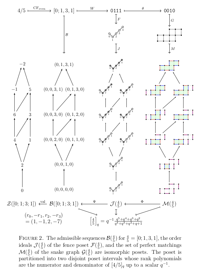
At the end of the introduction of our preprint, Figure 2 shows an illustration of our three combinatorial interpretations for the q-analog of the rational number 4/5
\(\left[\frac{4}{5}\right]_q = q^{-1}\frac{q^5+q^4+q^3+q^2}{q^4+q^3+q^2+q+1}\)
which is reproduced below:
The number 4/5 is just one very small example. But our result works for all positive rational numbers.
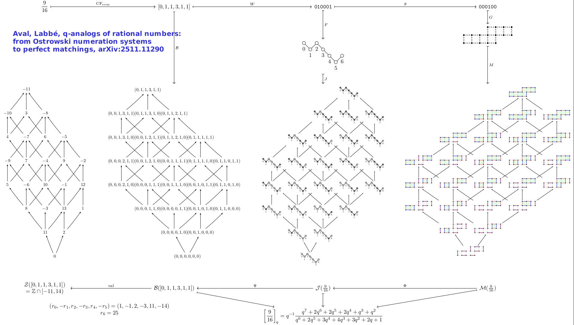
Here is the same Figure made for 9/16:
\(\left[\frac{9}{16}\right]_q=q^{-1}\frac{q^{7} + 2q^{6} + 2q^{5} + 2q^{4} + q^{3} + q^{2}}{q^{6} + 2q^{5} + 3q^{4} + 4q^{3} + 3q^{2} + 2q + 1}\)
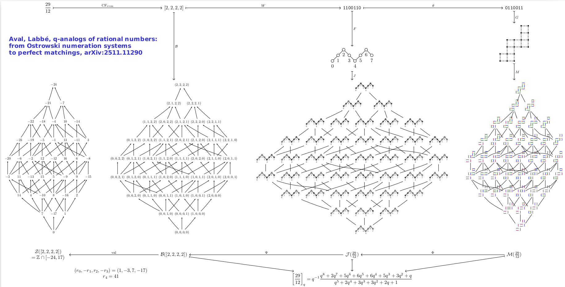
Here is the same Figure made for 29/12:
\(\left[\frac{29}{12}\right]_q=q^{-1}\frac{q^{8} + 2q^{7} + 5q^{6} + 6q^{5} + 6q^{4} + 5q^{3} + 3q^2 + q}{q^{5} + 2q^{4} + 3q^{3} + 3q^{2} + 2q + 1}\)
The above two images are available for download as pdf here:
- A pdf illustrating \([9/16]_q\)
- A pdf illustrating \([29/12]_q\)
- A 31 pages pdf of the first 31 rational numbers up to depth 4 in the Stern-Brocot tree (a phantom version of the same document to be completed as an exercise)
I plan to make by code public soon in my SageMath package slabbe in order for anyone to reproduce any of these figures for every positive rational number. Perhaps, I will do this during the next Sage Days in Montreal.
NOTE: There is a typo in our version v1 of the preprint available on arxiv. In the definition of the function F from binary words to fence posets, the letters 0 and 1 should be swapped: letter 1 means a up-step and letter 0 means a down step. We will fix the typo together with other changes to be made during the review process. The typo is strange because it means we are not consistent with the notation of the recent article of McConville, Propp and Sagan published in Forum of Math, Sigma. This is something which we will investigate further during the review process.
A construction of the hat tilings by a Markov partition
26 mars 2026 | Mise à jour: 06 mai 2026 | Catégories: math | View CommentsOn October 3rd, 2025, in Montreal, Peter Selinger gave a talk at LaCIM in Montreal (where I am based this year in the French IRL CRM-CNRS laboratory) about the hex game. After lunch, I asked him to play against him. Since I needed to leave in about 30 minutes to give a colloquim at CRM at Université de Montréal, I thought playing againt Peter should not take too long as I would lose fast.
We ended up never even starting the hex game.
Peter was also short in time because he was also giving a second seminar the same day in the afternoon this time at McGill University about Quantum computing, his main research subject.
Peter asked me what was my talk about. I said aperiodic tilings associated to the metallic mean, etc. Then, he showed me a picture he recently made. Right away, I recognized the fractal shape in the partition of the internal space described by Baake, Gähler and Sadun for tilings by the meta-tiles T, H, P and F following the original terminology of Smith, Myers, Kaplan and Goodman-Strauss. I was wondering since then if we could use their partition to describe the hat tilings the same way I did it for Jeandel-Rao tilings. So, I asked Peter how he got the picture. Then he told me exactly what I was hoping for. Peter's construction is marvelous!
With the semester Illustration as a mathematical research technique currently taking place this winter at Institut Henri Poincaré, Paris, I thought it would be a good occasion to share Peter's discovery. Together, we have been preparing a preprint presenting a construction of the hat tilings by a Markov partition following the approach I used in my work on Jeandel-Rao tilings. The preprint is not ready yet to be posted on arxiv, but we publicly share our draft today, March 26th, 2026.
An important aspect of the construction is the choice made by Peter for the placement of the anchors for each tile. Anchors are widely and commonly called control point in the community, but since Peter is an expert on Bezier curves, the terminology of control point did not make sense for him. And maybe he has a (control?) point.
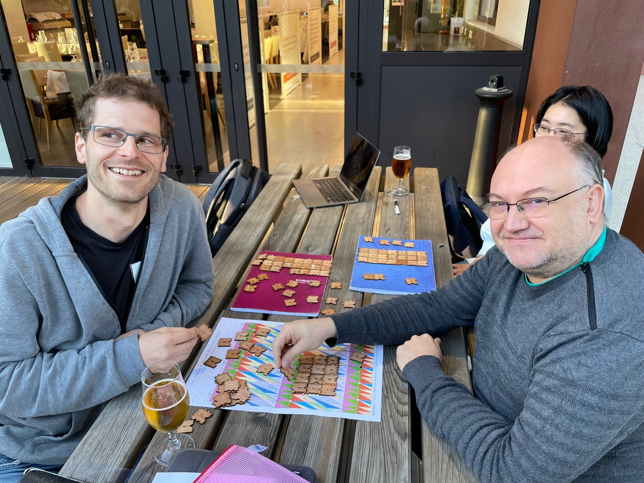
The partition discovered by Peter can be seen as a extension of what happens with Jeandel Rao tilings that I now explain visually with a DIY laser cut puzzle on top of a partition.
The talk at IHP on March 26 was recorded and will be available on the carmin.tv website.
UPDATE (April 24th, 2026): Our preprint is now online at arXiv:2604.20964.
Here is additional documents to produce hat tilings from the placement of a transparent grid on top of the partition. These DIY documents can be used for outreach activities (it works great!):
- solution_16x17.svg: a svg of a hat tiling to laser cut many hats
- grid-triangular-A4.pdf: the triangular grid in A4 format to be printed on acetate
- grid-triangular-letter.pdf: the triangular grid in letter format to be printed on acetate
- poster-partition-A3.pdf: the partition in A3 format
- poster-partition-A4.pdf: the partition in A4 format
- poster-partition-letter.pdf: the partition in letter format
All of the above documents use \(2\sqrt{3}\) cm for 1 unit corresponding to 3 cm for the height of the equilateral triangles in the grid. This is the choice I have made in 2023 when I made my first laser cut of the hats.
Now, I think using 3 cm would be better for the unit (side length of the equilateral triangles). Maybe next time I laser cut 1000 hat tiles, I will use this smaller size instead. If I do this one day, I will upload these new documents here.
UPDATE (May 6th, 2026): My coauthor Peter Selinger made an applet to put tiles on top of the Markov partition:
Découpe laser de pentagones qui pavent le plan
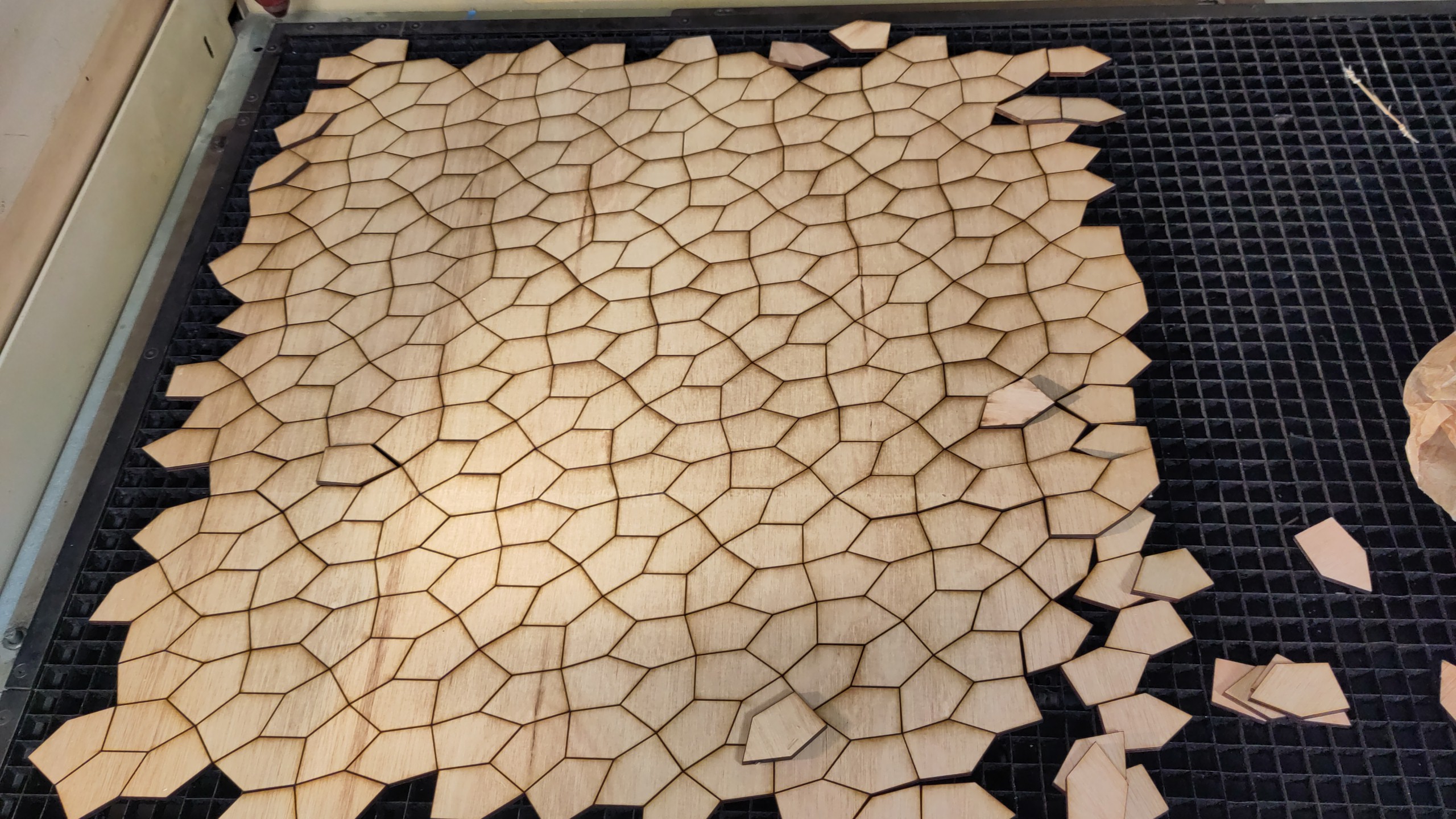
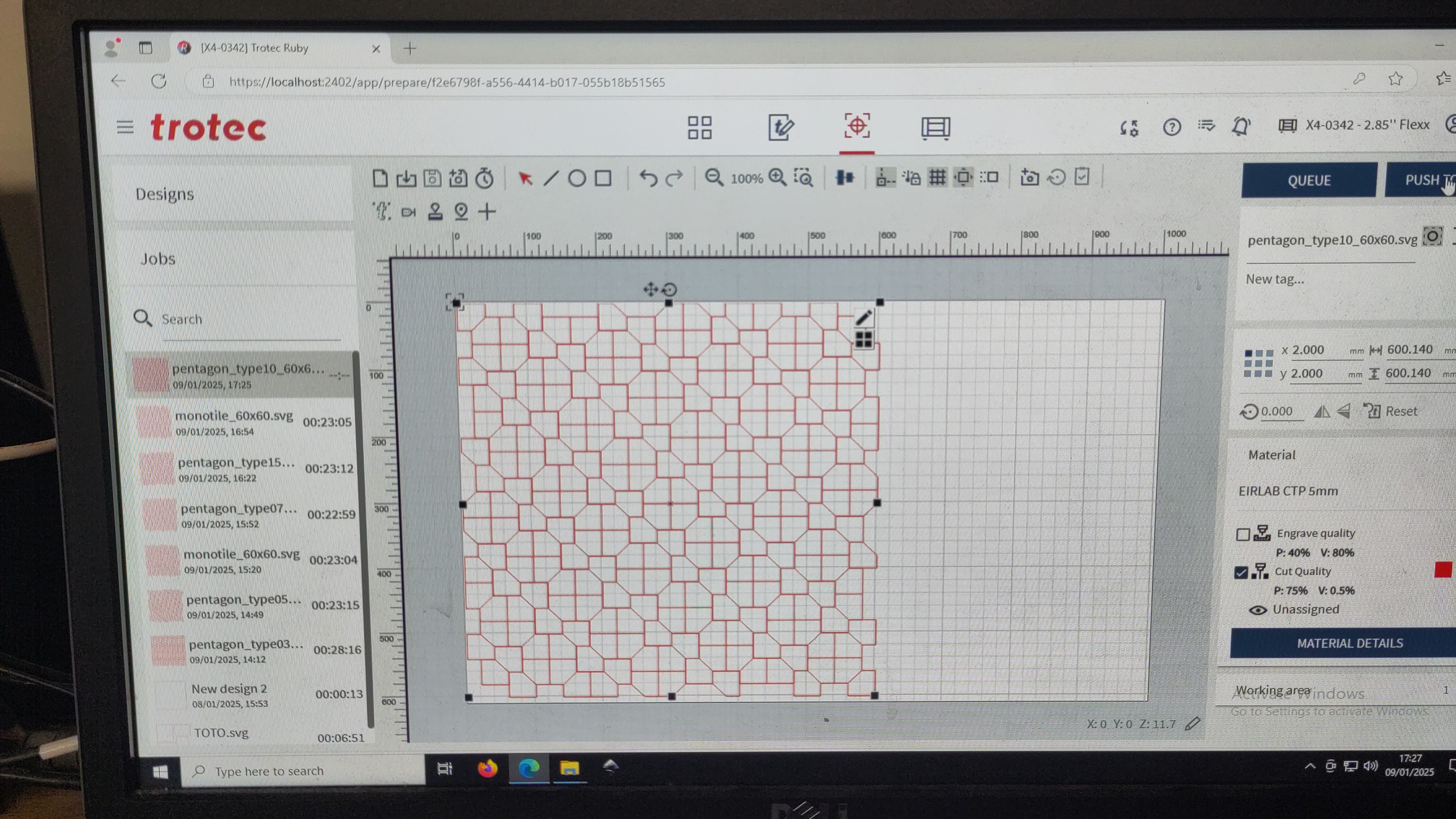
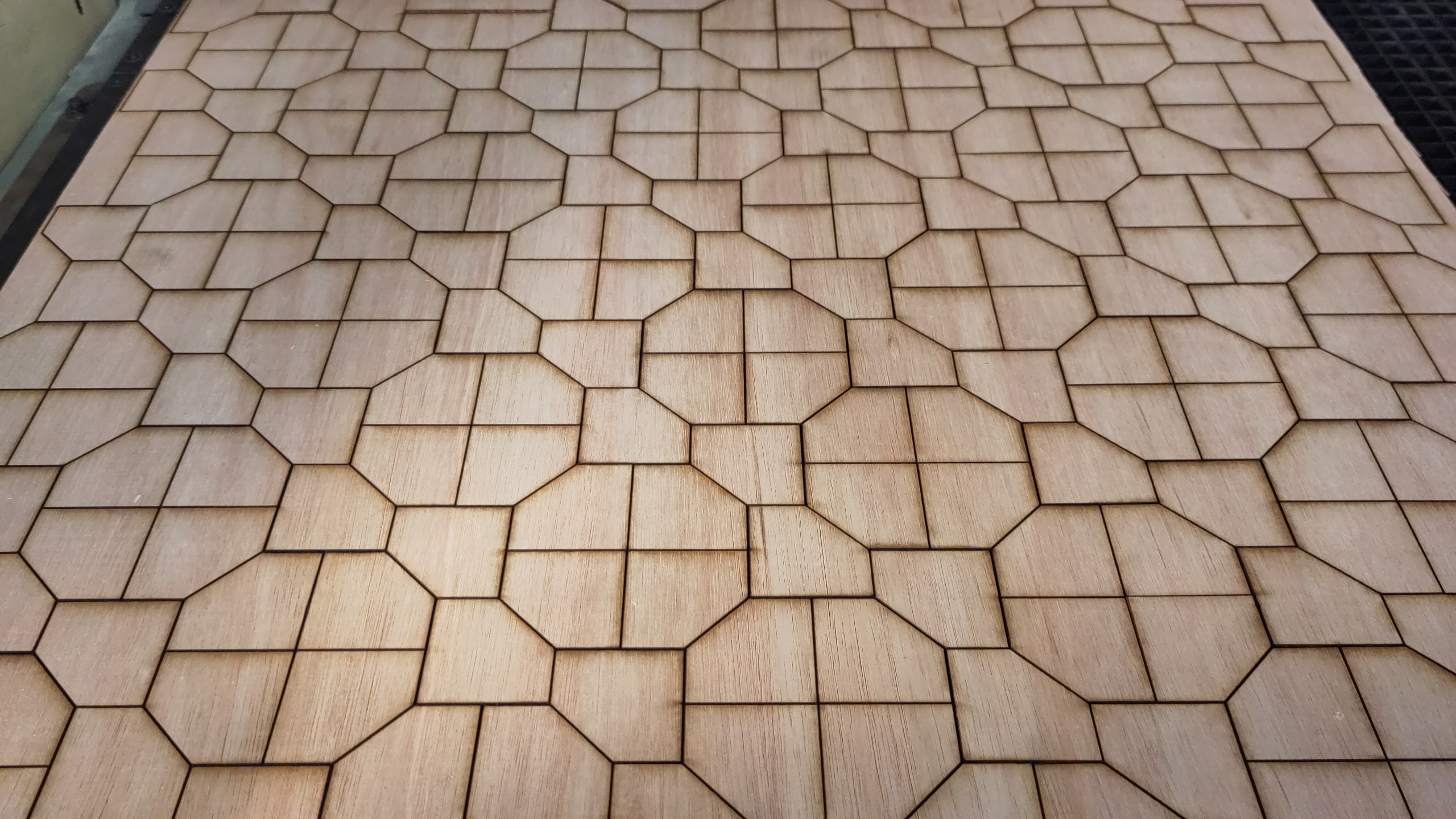
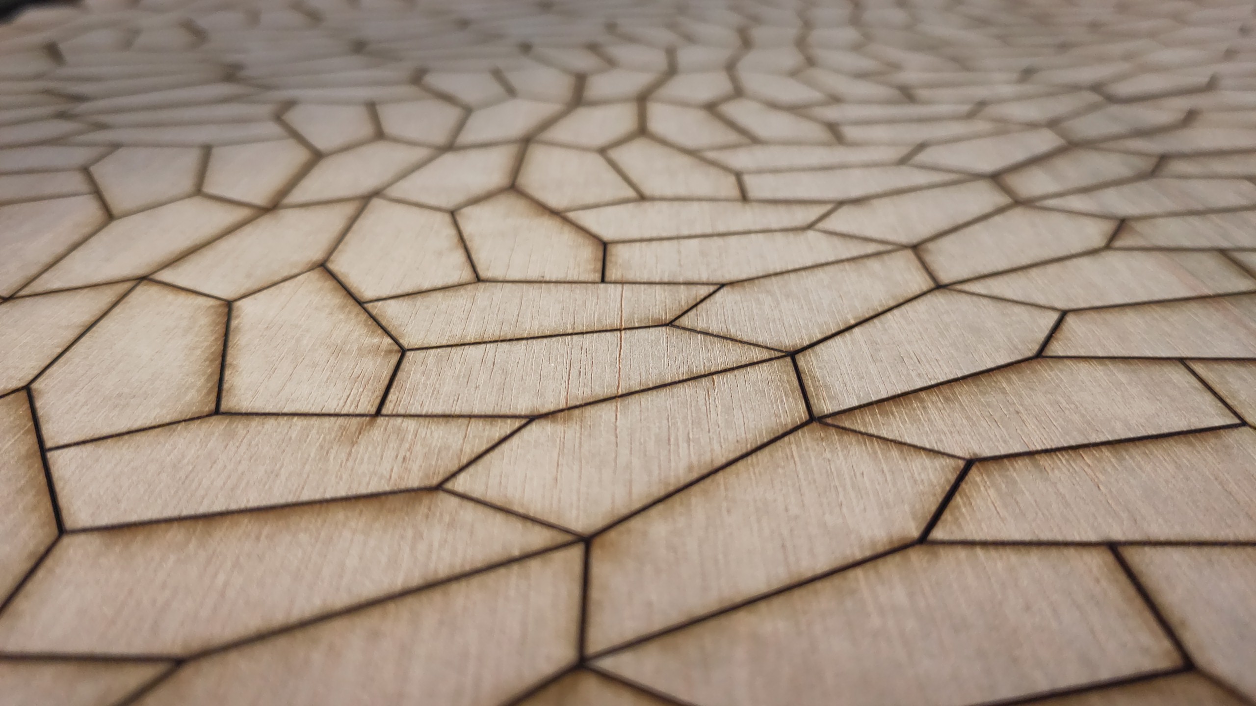
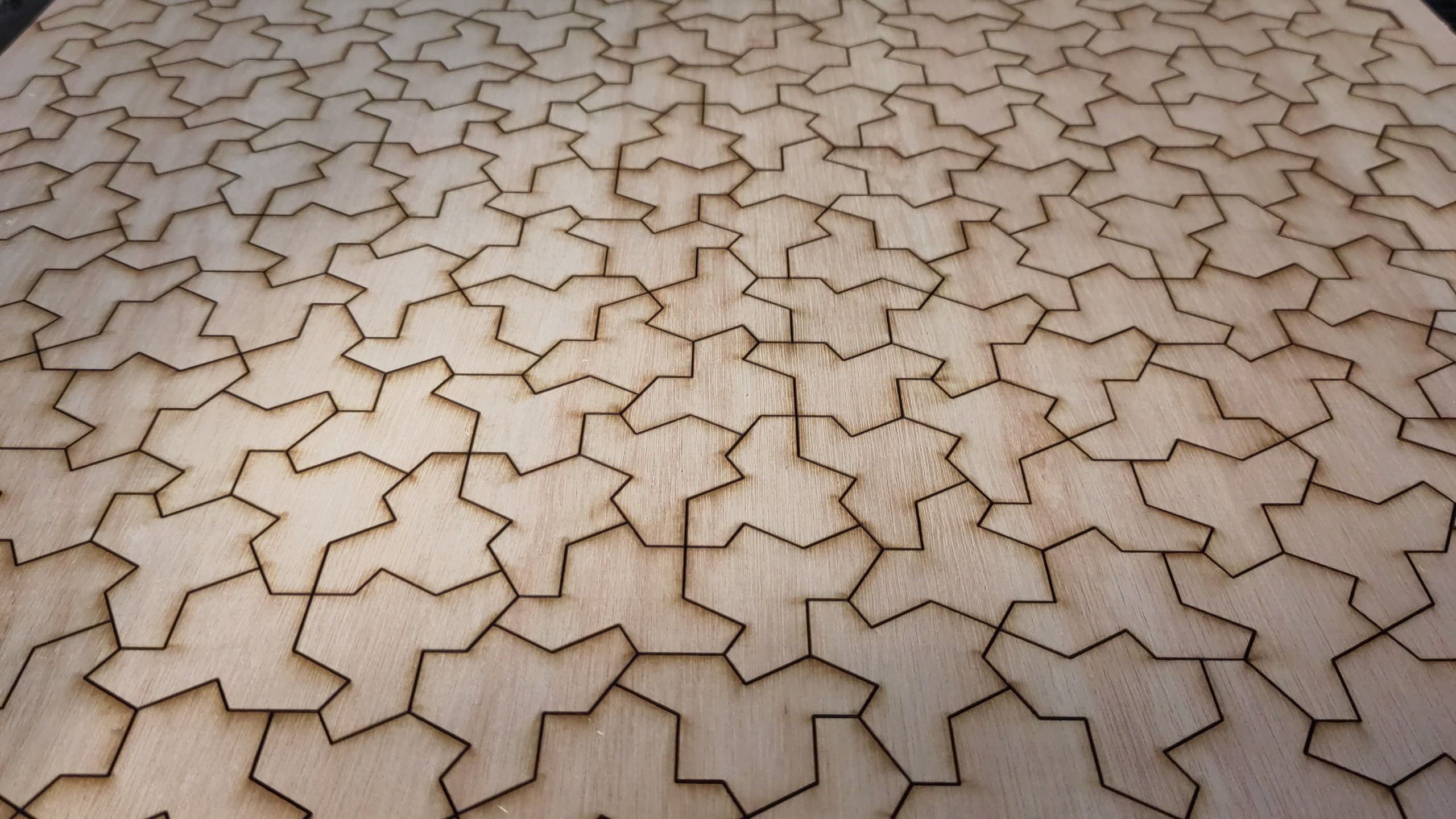
15 mai 2025 | Catégories: découpe laser, math | View CommentsEn janvier 2025, avec l'aide de David Renault, j'ai fait une nouvelle série de découpes lasers au fablab EirLab de l'ENSEIRB sur le thème des pavages par pentagones. Comme démontré par Michael Rao, il n'existe que 15 pavages pentagonaux possibles.
Voici quelques images de la découpe effectuée le 9 janvier 2025.
Un pentagone de type 7 découvert par Kershner en 1968:
Un pentagone de type 10 découvert par James en 1975:
Le pentagone de type 15 découvert en 2015 par Jennifer McLoud-Mann, Casey Mann et David Von Derau, un étudiant de niveau licence en stage avec eux:
J'ai pu rencontrer Casey et Jennifer pour la première fois en 2017 à Montréal. Ils ont passé une année sabbatique à l'Université de Bordeaux en 2019-2020 via le programme Visiting Scholar de l'Université de Bordeaux, et cela a mené à une publication scientifique commune.
J'en ai aussi profité pour découper quelques tuiles chapeau apériodiques en plus:
Interventions dans les collèges et lycées en Gironde
Ces dernières années, sous l'invitation annuelle de Johanne Brengues, professeure au Lycée Kastler, j'ai développé un atelier sur la structure des flocons de neige et pavages apériodiques. Dans l'atelier d'une durée de 60 à 120 minutes, j'utilise des pièces en bois découpées au laser à l'ENSEIRB pour faire découvrir la science des pavages apériodiques et des quasicrystaux par la manipulation.
Pour l'année 2024-2025, j'ai soumis l'atelier suivant à l'Académie de Bordeaux dans le cadre de l'activité Des universitaires dans les classes.
Titre: Structure des flocons de neige et pavages apériodiques
Résumé: On dit que les flocons de neige sont tous différents. Pourquoi alors les branches d’un même flocon sont identiques? Dans cet exposé interactif, nous étudierons ces questions du point de vue des pavages du plan par des pièces de puzzle polygonales. Ces pièces se collent les unes aux autres comme le font en trois dimensions les molécules d’eau lors de la formation d’un flocon. En particulier, nous manipulerons des dizaines de copies d’un polygone à 13 côtés découvert en mars 2023. Les copies de ce polygone ont la propriété de paver le plan sans jamais se répéter. Nous utiliserons cet exemple pour discuter des pavages apériodiques du plan et de leurs propriétés. Public : tout niveau primaire + collège + lycée
J'ai été contacté par plusieurs collèges de la région pour faire cet atelier au printemps 2025:
- Collège Cassignol Bordeaux, 28 élèves de 3e, 7 janvier 2025
- Collège Jean Rostand, Casteljaloux, 3 classes de 6e, 16 janvier 2025
- Collège Olympe de Gouges, Vélines, 17 janvier 2025
- Village de maths, Collège Laure Gatet, Périgueux, 13 mars 2025
- Lycée Kastler, Talence, 15 mai 2025
- Collège Jean Zay, Cenon, 13 juin 2025
Les professeurs me disent que les pavages sont au programme du collège ce qui facilite les liens avec le sujet de l'atelier.
L'atelier en 2024-2025
Dans mes recherches, je m'intéresse à la combinatoire et à ses interactions avec les autres sciences. Par exemple, les atomes se combinent pour former des molécules stables en suivant des règles combinatoires simples. À l'état solide, les molécules peuvent se combiner pour former des structures ordonnées comme des crystaux ou même des flocons de neige.
La structure des flocons de neige est une science passionnante étudiée par Kenneth Libbrecht, professeur de physique au California Institute of Technology. Plusieurs questions naturelles peuvent-être posées par les élèves en voyant quelques images de flocons de neige:
- Pourquoi les flocons ont tous 6 branches?
- Pourquoi les branches d'un même flocon sont pareilles?
Après l'introduction sur la combinatoire et les flocons de neige, on passe à l'atelier. On divise la classe en petits groupes de 3 à 5 élèves. On attribue un atome (c'est-à-dire, plusieurs copies d'un même polygone) à chaque groupe. On demande aux élèves de trouver les molécules que l'atome peut créer en deux dimensions. On oriente les élèves à trouver des grandes molécules qui recouvrent des disques arbitrairement grand (on demande de recouvrir une feuille format A7, puis format A6, puis format A5, puis format A4).
Comme les pavages pentagonaux sont périodiques, nous démarrons l'atelier par l'exploration des pavages par l'un des 15 types de pentagones qui pavent le plan. Chaque groupe d'élèves se voit attribuer plusieurs copies d'une sorte de pentagones. Les élèves doivent explorer la combinatoire de la forme géométrique et faire des observations. Les découvertes des élèves sont publiées au tableau pendant l'atelier comme un article scientifique. Les résultats publiés peuvent être utilisés par les autres groupes à condition de les citer!
La notion d'apériodicité se transmet mieux après avoir compris la notion de pavages périodiques. La nouveauté pour mon atelier du printemps 2025 était de faire en sorte que les élèves découvrent d'abord des pavages périodiques non triviaux avant de considérer des pavages apériodiques. Cela permet de mieux expliquer la notion d'apériodicité.
Toutefois, avec une introduction de 15 à 20 minutes, l'atelier sur les pentagones nécessite presque la totalité du temps restant (30 minutes). Dans certains cas, un des groupes peut commencer l'étude de la pièce apériodique chapeau dans les 10 minutes restantes. Dans d'autres situations, je laisse un groupe choisir la pièce chapeau dès le début de l'atelier. Quand le temps le permet, on peut prévoir l'atelier en deux périodes de 60 minutes avec le même groupe. Cela permet d'explorer les pièces pentagonales périodiques, puis les pièces apériodiques tout en laissant du temps pour répondre aux questions des élèves.
Voici des fichiers qui rassemblent les images que j'utilise dans l'atelier sur les différents thèmes présentés.
Voici quelques liens pour en savoir plus:
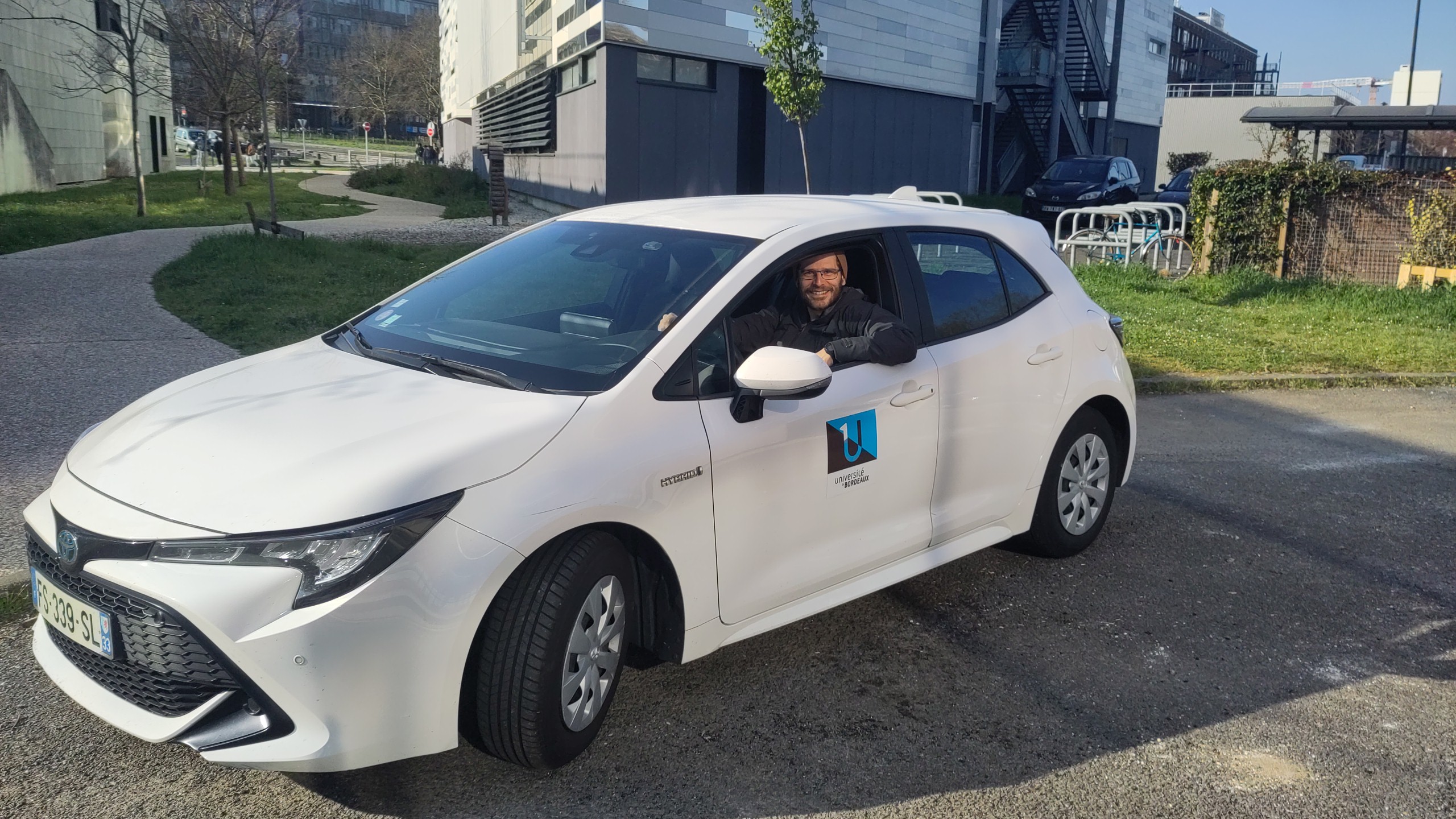
Pour les collèges et lycées en dehors de Bordeaux et difficilement accessible en transport en commun, je remercie l'Université de Bordeaux pour le prêt d'une voiture.
On the bifurcation diagram proposed by Jang and Robinson
06 mai 2025 | Catégories: sage, math | View CommentsIn this blog post, we present a few remarks on the "bifurcation diagram" proposed by Jang and Robinson in [1] to describe the tilings associated to a set of 24 Wang tiles encoding Penrose tilings.
[1] Hyeeun Jang, E. Arthur Robinson Jr, Directional Expansiveness for Rd-Actions and for Penrose Tilings, arxiv:2504.10838
In particular, I believe that something is wrong in what the authors call the "bifurcation diagram" shown in Figure 10. But, as we illustrate below, it can be fixed easily by permuting some of the labels of the partition.
I saw Jang and Robinsion's bifurcation diagram for the first time during the talk "Remembering Shunji Ito" made by Robinson during the online conference dedicated to the memory of Shunji Ito on December 14, 2021. At that time, I was working on the family of metallic mean Wang tiles. This is why the bifurcation diagram shown by Robinson and extracted from Jang's PhD thesis got my attention right away, because it was looking very much like the Markov partition associated to the Ammann set of 16 Wang tiles, the first member of the family of metallic mean Wang tiles. As we illustrate below, Jang and Robinson's bifurcation diagram is a refinement of the Markov partition associated the Ammann set of 16 Wang tiles. This means that the 16 tiles Ammann Wang shift is a factor of the 24 tiles Penrose Wang shift. Also most probably the bifurcation diagram is a Markov Partition for the same associated toral ℤ2-action. But this needs a proof.
The content of this blog post is also available as a Jupyter notebook that can be viewed and downloaded from the nbviewer.
Dependencies
The computations made here depend on the modules WangTileSet, WangTiling, PolyhedronPartition, PolyhedronExchangeTransformation, PETsCoding implemented in the SageMath optional package slabbe over the last years in order to describe and study the Jeandel-Rao aperiodic tilings and the family of metallic mean Wang tiles.
Note that the package slabbe can be installed by running !pip install slabbe directly in SageMath:
sage: # !pip install slabbe # uncomment and execute this line to install slabbe package
Here are the version of the packages used in this post:
sage: import importlib
sage: importlib.metadata.version("slabbe")
'0.8.0'
sage: version()
'SageMath version 10.5.beta6, Release Date: 2024-09-29'
Jang-Robinson encoding of the Penrose 24 Wang tiles
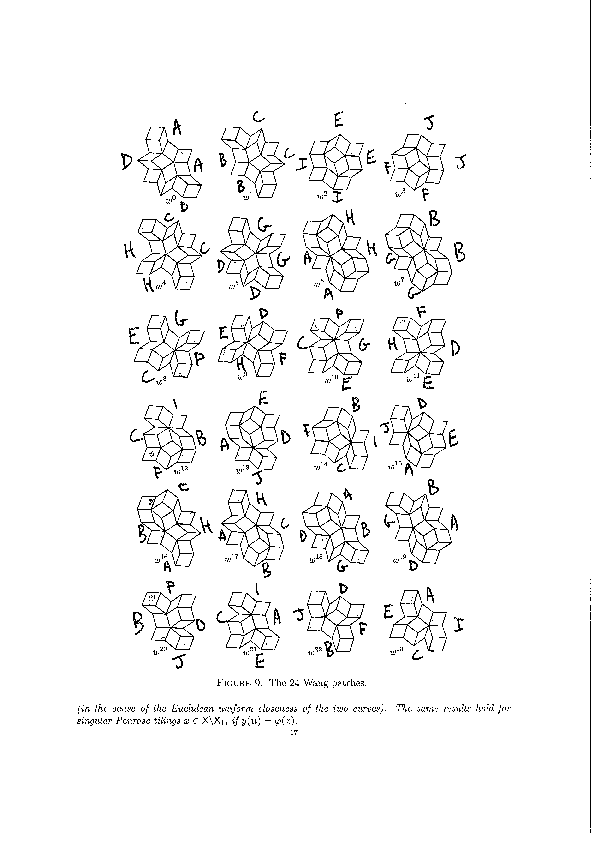
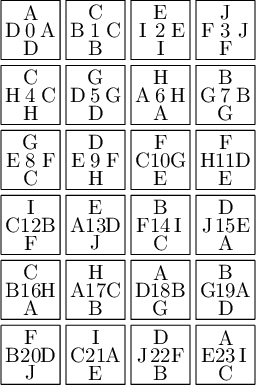
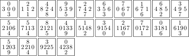
We encode the 24 Wang tiles proposed by Jang and Robinson (Figure 9 of [1]) using alphabet {A, B, C, D, E, F, G, H, I, J} for the shapes:
We define the 24 Wang tiles in SageMath:
sage: from slabbe import WangTileSet, WangTiling
sage: tiles = ["AADD", "CCBB", "EEII", "JJFF",
....:          "CCHH", "GGDD", "HHAA", "BBGG",
....:          "FGEC", "FDEH", "GFCE", "DFHE",
....:          "BICF", "DEAJ", "IBFC", "EDJA",
....:          "HCBA", "CHAB", "BADG", "ABGD",
....:          "DFBJ", "AICE", "FDJB", "IAEC"]
sage: T0 = WangTileSet([tuple(str(a) for a in tile) for tile in tiles])
sage: T0
Wang tile set of cardinality 24
sage: T0.tikz(ncolumns=4)
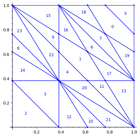
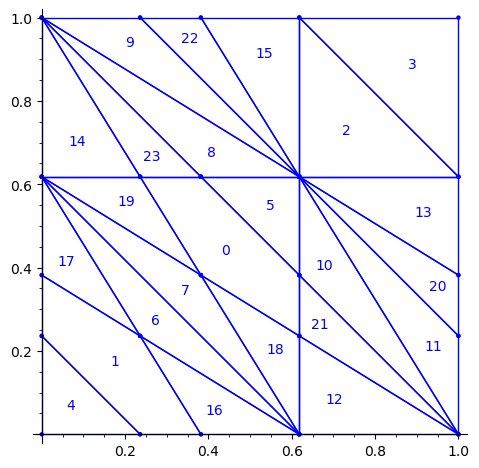
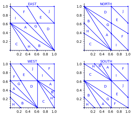
Constructing Jang-Robinson Bifurcation diagram as a polygonal partition
Below is a reproduction of Jang-Robinson bifurcation diagram shown in Figure 10 from arxiv:2504.10838
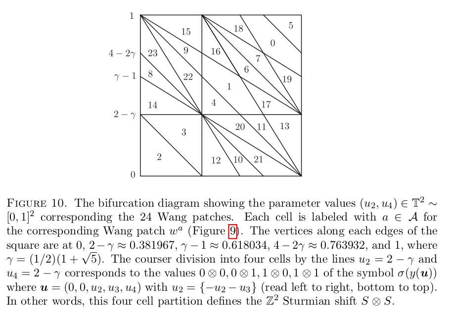
In this section, we construct this bifurcation diagram in SageMath as a polygonal partition.
sage: from slabbe import PolyhedronPartition
sage: z = polygen(QQ, 'z')
sage: K = NumberField(z**2-z-1, 'phi', embedding=RR(1.6))
sage: phi = K.gen()
sage: square = polytopes.hypercube(2,intervals = 'zero_one')
sage: P = PolyhedronPartition([square])
sage: P = P.refine_by_hyperplane([1/phi^3,-1,-1])
sage: P = P.refine_by_hyperplane([1/phi,-1,-1])
sage: P = P.refine_by_hyperplane([1,-1,-1])
sage: P = P.refine_by_hyperplane([1 + 1/phi,-1,-1])
sage: P = P.refine_by_hyperplane([1 + 1/phi^3,-1,-1])
sage: P = P.refine_by_hyperplane([1/phi,-phi,-1])
sage: P = P.refine_by_hyperplane([1,-phi,-1])
sage: P = P.refine_by_hyperplane([phi,-phi,-1])
sage: P = P.refine_by_hyperplane([1/phi^2,-1/phi,-1])
sage: P = P.refine_by_hyperplane([1/phi,-1/phi,-1])
sage: P = P.refine_by_hyperplane([1,-1/phi,-1])
sage: P = P.refine_by_hyperplane([1/phi,-1,0])
sage: P = P.refine_by_hyperplane([1/phi,0,-1])
sage: P = -P
sage: P = P.translate((1,1))
sage: #P.plot()
sage: P = P.rename_keys({0:5, 1:0, 2:18, 3:19, 4:7, 5:6, 6:16, 7:17, 8:1, 9:4, 10:15,11:9,
sage:                    12:22,13:23,14:8, 15:14,16:13,17:11,18:20,19:21,20:10, 21:12, 22:3,
sage:                    23:2})
sage: P.plot()
Our claim
We claim that the above bifurcation diagram from Jang-Robinson preprint is slightly wrong according to the choice of indices of the 24 Wang tiles made by Jang and Robinson and shown above. The following changes should be made in order to fix the partition:
- indices 9 and 22 should be swapped,
- indices 8 and 23 should be swapped,
- indices 11 and 20 should be swapped and
- indices 10 and 21 should be swapped.
Defining the toral translations in the internal space as PETs
We define the toral translations associated to the partition chosen by Jang-Robinson. The internal space is the 2-dimensional torus ℝ2 ⁄ ℤ2. It is represented as the unit square [0, 1)2. On this fundamental domain, a toral translation is a polygon exchange transformation.
Note that according to their choice,
- a unit horizontal translation in the physical space corresponds to a vertical translation by (0, φ) in the internal space,
- a unit vertical translation in the physical space corresponds to a horizontal translation by (φ, 0) in the internal space,
where φ is the golden mean.
Below, we follow their convention.
sage: from slabbe import PolyhedronExchangeTransformation as PET
sage: base = diagonal_matrix((1,1))
sage: R0e1 = PET.toral_translation(base, vector((0,phi)))
sage: R0e2 = PET.toral_translation(base, vector((phi,0)))
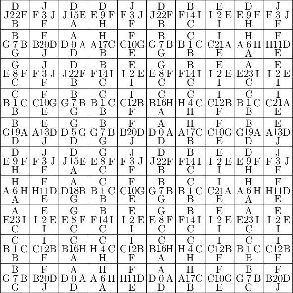
We compute a 10×10 pattern obtained by coding the orbit of some starting point under the ℤ2-action R0.
sage: from slabbe.coding_of_PETs import PETsCoding
sage: coding_R0_P = PETsCoding((R0e1,R0e2), P)
sage: pattern = coding_R0_P.pattern((.3,.4), (10,10))
sage: pattern = WangTiling(pattern, T0)
sage: pattern.tikz()
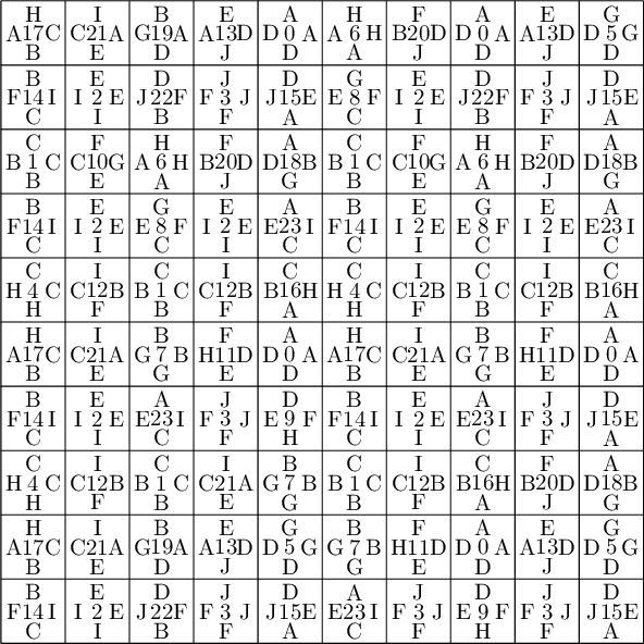
We observe that this pattern is not valid !!!
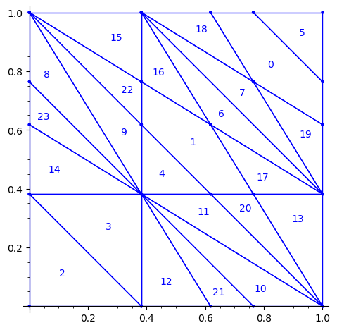
Let's fix the partition
We claim that the above pattern is wrong because something is wrong in the labelling of the atoms in the partition proposed by Jang and Robinson for the 24 Wang tiles encoding Penrose tilings.
Below, we fix the partition by swapping labels 8 and 23, 9 and 22, 11 and 20, 10 and 21:
sage: d = {i:i for i in range(24)}
sage: d.update({8:23, 23:8, 9:22, 22:9, 11:20, 20:11, 10:21, 21:10})
sage: P1 = P.rename_keys(d)
sage: P1.plot()
We compute a 10×10 pattern out of this updated partition P1:
sage: coding_R0_P1 = PETsCoding((R0e1,R0e2), P1)
sage: pattern = coding_R0_P1.pattern((.3,.4), (10,10))
sage: pattern = WangTiling(pattern, T0)
sage: pattern.tikz()
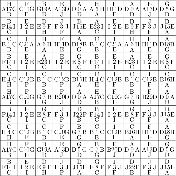
We observe that this pattern is valid !!!
Understanding the issue using edge label partitions
Let us try to understand the fix in terms of the Wang tiles east, north, west and south edge labels partitions induced by the original partition.
Indeed, since each atom of the partition corresponds to a Wang tile, we can deduce a partition of the unit square for the east labels (and respectively for the north, west and south labels) by merging two atoms in the partition if their east edge label is the same.
sage: def edge_label_partitions(partition, tiles):
....:     EAST = partition.merge_atoms({i:tiles[i][0] for i in range(24)})
....:     NORTH = partition.merge_atoms({i:tiles[i][1] for i in range(24)})
....:     WEST = partition.merge_atoms({i:tiles[i][2] for i in range(24)})
....:     SOUTH = partition.merge_atoms({i:tiles[i][3] for i in range(24)})
....:     return EAST, NORTH, WEST, SOUTH
sage: def draw_edge_label_partitions(partition, tiles):
....:     EAST, NORTH, WEST, SOUTH = edge_label_partitions(partition, tiles)
....:     L = [EAST.plot() + text('EAST', (.5,1.05)),
....:          NORTH.plot() + text('NORTH', (.5,1.05)),
....:          WEST.plot() + text('WEST', (.5,1.05)),
....:          SOUTH.plot() + text('SOUTH', (.5,1.05))]
....:     return graphics_array(L, nrows=2)
This is what we get using the partition proposed by Jang and Robinson for the 24 Wang tiles encoding Penrose tilings:
sage: draw_edge_label_partitions(P, T0)
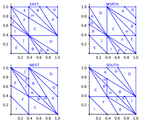
Here are some observations which are normal:
- partitions NORTH and EAST are symmetric under a reflexion by the positive diagonal (remember that the tile set is symmetric under the positive diagonal)
- partitions WEST and SOUTH are symmetric under a reflexion by the positive diagonal (remember that the tile set is symmetric under the positive diagonal)
Here are some observations which are not normal:
- partitions WEST and EAST do not give the same area to the same index (in a Wang tiling, the frequency of a EAST label should be equal to the frequency of the same WEST label)
- partitions SOUTH and NORTH do not give the same area to the same index (in a Wang tiling, the frequency of a NORTH label should be equal to the frequency of the same SOUTH label)
- partitions EAST and WEST are not a translate of one another (idealy a horizontal translate)
- partitions SOUTH and NORTH are not a translate of one another (idealy a vertical translate)
Another indication that something may be wrong is:
- atoms B, H, E, J, A, G are not convex in the torus
This is not a necessity. Atoms are not convex in the Markov partition associated to Jeandel-Rao tilings [2]. But they are convex for the Ammann set of 16 Wang tiles and their generalization to metallic mean numbers made in [3,4]. Since Penrose tilings are closely related to Ammann A2 tilings, we may also expect to have simple convex atoms in each of the four edge label partitions.
Here is the area of each atom in each of the four partitions. We observe that only atoms C and D have the same area in each of the four partitions.
sage: def table_of_area_of_atom_in_east_north_west_south_partitions(partition, tiles):
....:     columns = []
....:     labels = 'ABCDEFGHIJ'
....:     EAST, NORTH, WEST, SOUTH = edge_label_partitions(partition, tiles)
....:     for partition in [EAST, NORTH, WEST, SOUTH]:
....:         d = partition.volume_dict()
....:         column = [d[a] for a in labels]
....:         columns.append(column)
....:     header_row = ['EAST', 'NORTH', 'WEST', 'SOUTH']
....:     return table(columns=columns, header_row=header_row, header_column=['']+list(labels))
sage: table_of_area_of_atom_in_east_north_west_south_partitions(P, T0)
    │ EAST             NORTH            WEST             SOUTH
├───┼────────────────┼────────────────┼────────────────┼────────────────┤
  A │ 15/2*phi - 12    15/2*phi - 12    phi - 3/2        phi - 3/2
  B │ phi - 3/2        phi - 3/2        15/2*phi - 12    15/2*phi - 12
  C │ phi - 3/2        phi - 3/2        phi - 3/2        phi - 3/2
  D │ phi - 3/2        phi - 3/2        phi - 3/2        phi - 3/2
  E │ phi - 3/2        phi - 3/2        -11/2*phi + 9    -11/2*phi + 9
  F │ -11/2*phi + 9    -11/2*phi + 9    phi - 3/2        phi - 3/2
  G │ -8*phi + 13      -8*phi + 13      -3/2*phi + 5/2   -3/2*phi + 5/2
  H │ -3/2*phi + 5/2   -3/2*phi + 5/2   -8*phi + 13      -8*phi + 13
  I │ 5*phi - 8        5*phi - 8        -3/2*phi + 5/2   -3/2*phi + 5/2
  J │ -3/2*phi + 5/2   -3/2*phi + 5/2   5*phi - 8        5*phi - 8
But, we observe that we can fix the partitions if we assume that the atoms C and D in the four partitions are correct. There is a unique translation sending atoms C,D in the partition WEST to the atoms C and D in the partition EAST. That translation should send the partition WEST exactly on EAST. Similarly for SOUTH and NORTH. This suggest a way to fix atoms B, H, E, J, A, G in the partition.
Fixed Edge labels partitions
Using the fixed partition, here is what we get.
sage: P1.plot()

sage: draw_edge_label_partitions(P1, T0)
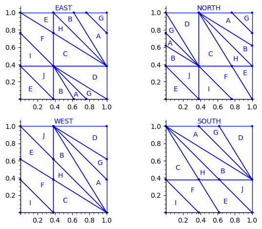
Now it looks good! As for the partitions associated to the metallic mean Wang tiles, the four partitions are isometric copies of the other ones (under toral translation or reflection).
sage: table_of_area_of_atom_in_east_north_west_south_partitions(P1, T0)
    │ EAST             NORTH            WEST             SOUTH
├───┼────────────────┼────────────────┼────────────────┼────────────────┤
  A │ phi - 3/2        phi - 3/2        phi - 3/2        phi - 3/2
  B │ phi - 3/2        phi - 3/2        phi - 3/2        phi - 3/2
  C │ phi - 3/2        phi - 3/2        phi - 3/2        phi - 3/2
  D │ phi - 3/2        phi - 3/2        phi - 3/2        phi - 3/2
  E │ phi - 3/2        phi - 3/2        phi - 3/2        phi - 3/2
  F │ phi - 3/2        phi - 3/2        phi - 3/2        phi - 3/2
  G │ -3/2*phi + 5/2   -3/2*phi + 5/2   -3/2*phi + 5/2   -3/2*phi + 5/2
  H │ -3/2*phi + 5/2   -3/2*phi + 5/2   -3/2*phi + 5/2   -3/2*phi + 5/2
  I │ -3/2*phi + 5/2   -3/2*phi + 5/2   -3/2*phi + 5/2   -3/2*phi + 5/2
  J │ -3/2*phi + 5/2   -3/2*phi + 5/2   -3/2*phi + 5/2   -3/2*phi + 5/2
sage: (phi-3/2).n(), (-3/2*phi + 5/2).n()
(0.118033988749895, 0.0729490168751576)
Labels A, B, C, D, E and F all have the same frequency of ϕ − (3)/(2) ≈ 0.118.
Labels G, H, I and J all have the same frequency of − (3)/(2)ϕ + (5)/(2) ≈ 0.0729.
We check that frequencies sum to 1:
sage: 6 * (phi-3/2) + 4 * (-3/2*phi + 5/2)
1
Proposed partition for the encoding of the Penrose tilings into 24 Wang tiles
As done with the Markov partition associated to Jeandel-Rao aperiodic tilings, and for the Markov partition associated to the family of metallic mean Wang tiles, I think it is more natural to associate horizontal (vertical) translations in the internal space with horizontal (vertical) translations in the physical space. This way, the brain is less mixed up and the projections in the physical space π and in the internal space πint of the cut and project scheme are defined more naturally. This way the internal space and physical space can even be identified: this is the root of the do-it-yourself tutorial allowing the construction of Jeandel-Rao tilings [5]. See also my Habilitation à diriger des recherches written in English during Spring 2025 for more information [6].
First, we flip the partition P1 by the positive diagonal. This exchanges the role of x and y axis.
sage: P2 = P1.apply_linear_map(matrix(2, [0,1,1,0]))
sage: P2.plot()

This allows to define the ℤ2-action R1 on the torus with horizontal and vertical translations for e1 and e2 respectively:
sage: base = diagonal_matrix((1,1))
sage: R1e1 = PET.toral_translation(base, vector((1/phi,0)))
sage: R1e2 = PET.toral_translation(base, vector((0,1/phi)))
Then, we rotate the partition. This changes the origin of the partition. This change may be optional, but it makes the partition look closer to the partitions already studied in [2,3,4]. It simplifies the explanation of any relation between them (and there is one, see below!).
sage: P3 = R1e1(P2)
sage: P3 = R1e2(P3)
sage: P3.plot()
We observe that the partition P3 associated to the 24 Wang tiles encoding Penrose tiling is a refinement of the partition associated to the 16 Ammann tiles (see Figure 15 in [4] as the 16 Ammann tiles are equivalent to the n-th metallic mean Wang tiles when n = 1).
We compute a 10×10 pattern obtained by coding the orbit of some starting point under the ℤ2-action R1 using partition P3.
sage: from slabbe.coding_of_PETs import PETsCoding
sage: coding_R1_P3 = PETsCoding((R1e1,R1e2), P3)
sage: pattern = coding_R1_P3.pattern((.3,.4), (10,10))
sage: pattern = WangTiling(pattern, T0)
sage: pattern.tikz()
We are happy to see that the pattern is still valid after all the changes we have made!
sage: draw_edge_label_partitions(P3, T0)
We observe that the EAST, NORTH, WEST and SOUTH partitions are a refinement of the EAST, NORTH, WEST and SOUTH partitions associated to the Ammann tiles partition (see Figure 15 in [4]).
The difference between the Ammann EAST and 24 Wang tiles Penrose EAST partition is the addition of two closed geodesics of slope -1 on the 2-torus passing through the origin and through the vertex (0, φ − 1).
It is possible that there is a clever way of including this information into the labels of the Wang tiles as we have done it for the family of metallic mean Wang tiles. Possibly, we need to use 4-dimension vectors for the tile labels instead of 3-dimensional integer vectors. This remains an open question.
Wang tiles deduced from the partition and ℤ2-action
We check that the Wang tiles computed from the partition P3 and ℤ2-action R1 is the original set of 24 Wang tiles defined by Jang and Robinson.
See Proposition 8.1 in [2].
sage: T = coding_R1_P3.to_wang_tiles()
sage: T.tikz()
sage: T.is_equivalent(T0, certificate=True)
(True,
 {'3': 'D',
  '0': 'A',
  '6': 'G',
  '1': 'B',
  '7': 'H',
  '2': 'C',
  '8': 'I',
  '4': 'E',
  '5': 'F',
  '9': 'J'},
 {'3': 'D',
  '0': 'A',
  '6': 'G',
  '1': 'B',
  '7': 'H',
  '2': 'C',
  '8': 'I',
  '4': 'E',
  '5': 'F',
  '9': 'J'},
 Substitution 2d: {0: [[0]], 1: [[1]], 2: [[2]], 3: [[3]], 4: [[4]], 5:
 [[5]], 6: [[6]], 7: [[7]], 8: [[8]], 9: [[9]], 10: [[10]], 11: [[11]], 12:
 [[12]], 13: [[13]], 14: [[14]], 15: [[15]], 16: [[16]], 17: [[17]], 18: [[18]],
 19: [[19]], 20: [[20]], 21: [[21]], 22: [[22]], 23: [[23]]})
A do-it-yourself polygonal partition to construct Jeandel-Rao tilings
05 avril 2024 | Mise à jour: 07 février 2025 | Catégories: découpe laser, math | View CommentsIn 2015, Emmanuel Jeandel and Michael Rao discovered a very nice set of 11 Wang tiles which can be encoded geometrically into the following set of 11 geometrical shapes:
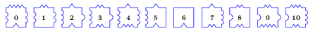
Jeandel and Rao proved that you may tile the plane with infinitely many translated copies of these tiles, but never periodically:
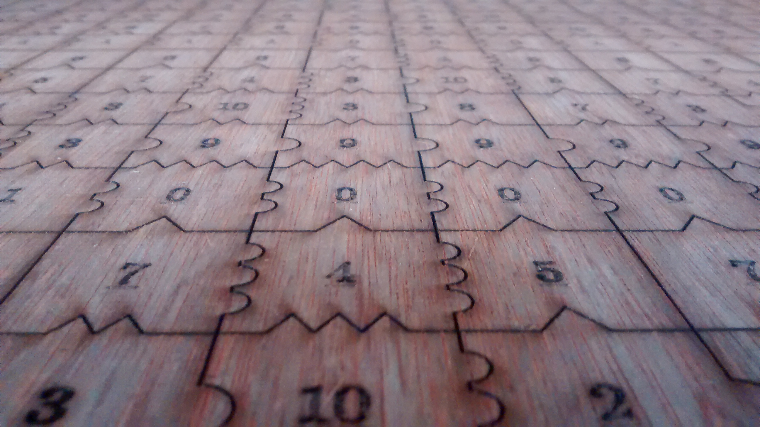
There is an easy way to construct Jeandel-Rao tilings from a well-chosen polygonal partition of the plane.
This is the polygonal partition:
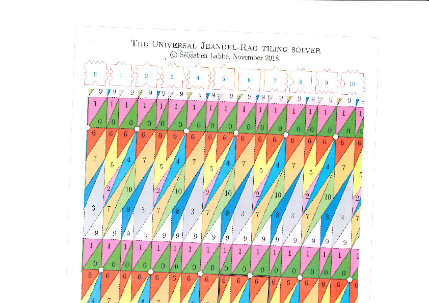
A lattice, represented below by the set of intersection of two perpendicular set of gridlines, is placed at a random position on top of the partition:
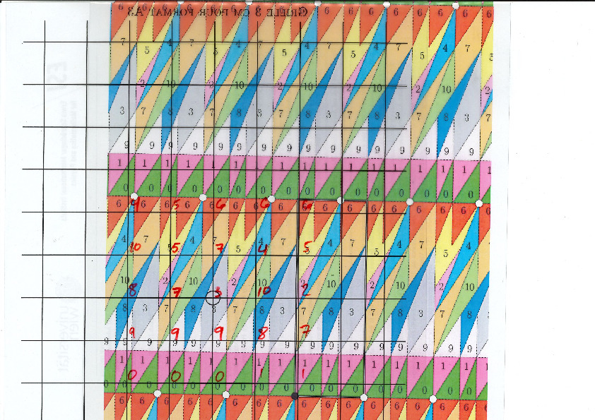
Each point of the lattice can be associated to an index from 0 to 10 according to which polygon of the partition it falls in. This defines a configuration of indices associated to each integer coordinate:
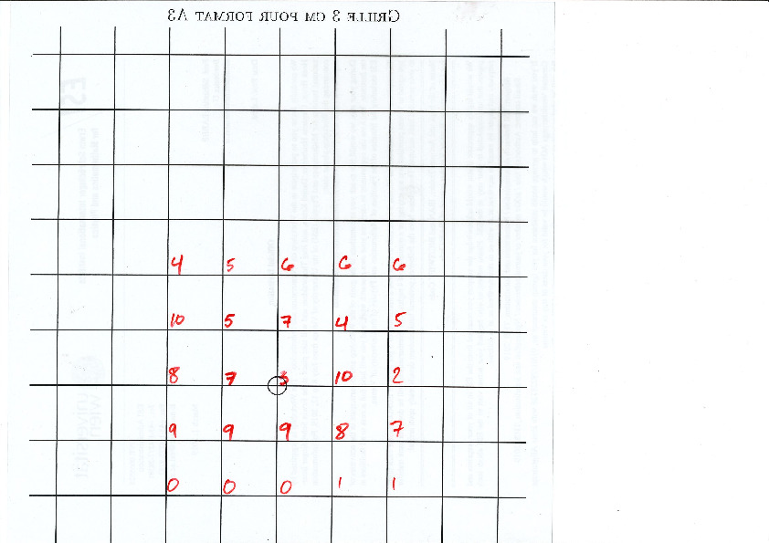
This procedure can be done all the way up to infinity. The chosen placement of the lattice defines a valid tiling of the plane with Jeandel-Rao tiles!

Since the size of the fundamental domain of the polygonal partition is irrational (width is golden mean, height is golden mean + 3, while the distance between two parallel gridlines is 1 unit), the generated configuration must be non-periodic.
It was a pleasure for me to do illustrate this to Emmanuel Jeandel during the workshop Multidimensional symbolic dynamics and lattice models of quasicrystals at CIRM in April 2024 in Marseille.
Do it yourself
Here are the files allowing to reproduce this experiment:
- A 33 x 19 rectangular valid patch of 627 tiles to use to cut a 1 meter x 60 cm wooden flat sheet (in svg format for laser cutting, pieces should have a side length of exactly 3 cm after the operation)
- The polygonal partition to be printed on a A3 paper (1 unit = 3 cm)
- The lattice \(\mathbb{Z}^2\) represented by gridlines 3cm apart to be printed on A4 paper (1 unit = 3 cm)
- A one-page Jeandel-Rao tiling solver tutorial
- A two-page document gathering the tutorial + partition (A4 paper format)
Alternate files for laser cutting the tiles
I first cut those tiles in August 2018 before a conference in Durham with the help of David Renault. We made more of them in June 2019. Each time David does some changes to the file that I provide to him with InkScape. Here are three alternate files for laser cutting the tiles.
Frequency of tiles
The frequency of tiles in a Jeandel-Rao tilings is computed below from the relative area in the associated polygonal partition. Tile #2 is the least frequent (around 2.55%) while tile #7 is the most frequent (around 15%):
sage: from slabbe.arXiv_1903_06137 import jeandel_rao_wang_shift_partition
sage: P0 = jeandel_rao_wang_shift_partition()
sage: V = P0.volume()
sage: tile_frequency = {a:v/V for (a,v) in P0.volume_dict().items()}
sage: rows = [(a, tile_frequency[a], tile_frequency[a].n(digits=3)) for a in range(11)]
sage: table(rows, header_row=['tile', 'frequency', 'frequency (numerical approx)'])
  tile   frequency           frequency (numerical approx)
├──────┼───────────────────┼──────────────────────────────┤
  0      -1/22*phi + 2/11    0.108
  1      -1/22*phi + 2/11    0.108
  2      9/22*phi - 7/11     0.0255
  3      -1/22*phi + 2/11    0.108
  4      2/11*phi - 5/22     0.0669
  5      -5/11*phi + 9/11    0.0828
  6      -1/22*phi + 2/11    0.108
  7      -3/11*phi + 13/22   0.150
  8      2/11*phi - 5/22     0.0669
  9      -1/22*phi + 2/11    0.108
  10     2/11*phi - 5/22     0.0669
When I construct a bag of 50 tiles of the Jeandel-Rao tiles, I follow the above tile frequencies. It yields:
sage: [(tile_frequency[a]*52).n(digits=3) for a in range(11)]
[5.63, 5.63, 1.33, 5.63, 3.48, 4.30, 5.63, 7.78, 3.48, 5.63, 3.48]
sage: [round(a) for a in _]
[6, 6, 1, 6, 3, 4, 6, 8, 3, 6, 3]
sage: sum(_)
52
Discussion
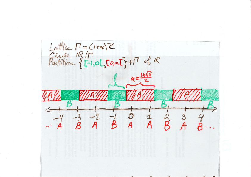
The construction of valid tilings with Jeandel-Rao tiles from a polygonal partition is a generalization of a well-known phenomenon in one dimension, namely, the fact that Sturmian sequences of complexity \(n+1\) are coded by irrational rotations. For example, here is an easy way to construct Sturmian sequences using a partition of the line into two intervals of different lengths. Similarly as above, every point from a set of equidistanced points is coded by letter A or B according to which of the two intervals it falls in.
The question that one may ask is whether all Jeandel-Rao tilings can be constructed from such a starting point in the partition. For Sturmian sequences, the answer is yes and the starting point can be described using the Ostrowski numeration system and the continued fraction expansion of the slope defined from the ratio of frequencies of the letters in the sequence. In one dimension, the proof is thus based on the desubstitution of Sturmian sequences on the one hand, and the Rauzy induction of irrational rotations on the other hand.
The same approach can be performed for Jeandel-Rao tilings using 2-dimensional desubstitution of Wang tilings and 2-dimensional Rauzy induction of toral \(\mathbb{Z}^2\)-rotations. Surprisingly, the two totally different methods applied on two completely different objects lead to the same sequence of eventually periodic 2-dimensional substitutions. Thus, every Jeandel-Rao tiling that can be desubstituted indefinitely can be constructed from the coding of some starting point in the polygonal partition.
Unfortunately, not all Jeandel-Rao tilings can be desubstituted indefinitely because of the existence of a horizontal fault line breaking the substitutive structure. Some configuration have a biinfinite horizontal row of the same tile labeled 0 in them. This allows to slide the lower half of configuration along the fault line and the configuration remains valid. A conjecture is that the remaining configurations are rare (of probability zero according to any shift-invariant probability measure). More precisely, I believe that all of the problematic ones can be described by a pair of starting points on the bottom segment of the polygonal partition. During the sabbatical year of Casey Mann and Jennifer Mcloud-Mann in Bordeaux in 2019-2020, we tried hard to prove that conjecture without success. It seems to be a difficult problem. Instead we described the nonexpansive directions in Jeandel-Rao tilings which reminds of the behavior of Penrose tilings with respect to Conway worms, their resolutions and essential holes (annulus of tiles which can be completed uniquely outside of the annulus, but not inside).
Aperiodic tilings related to the Metallic mean
The structure of Penrose aperiodic tilings, Jeandel-Rao aperiodic tilings and the new aperiodic hat monotile are all related to the golden mean. Do all aperiodic tilings need to be related to the golden ratio? What other numbers can be achieved?
During the conference at CIRM, I presented my newest result split into two parts: for every positive integer \(n\), there exists an aperiodic set of \((n+3)^2\) Wang tiles whose tiling structure is associated to the \(n\)-th metallic mean number, that is, the positive root of the polynomial \(x^2-nx-1\). This new discovery extends the knowledge we have on aperiodic tilings beyond the omnipresent golden ratio. The talk was recorded on youtube and the written notes are available here.
Jean-René Chazottes et Marc Monticelli
During the conference at CIRM, I met Jean-René Chazottes and Marc Monticelli. They made me know about their interactive online books, the outreach mathemarium website and its online experiments. Also, the Open-Fabrik-Maths fablab in Nice, including some experiments involving aperiodic Wang tilings.
Next Page »
Propulsé par Blogofile
S'abonner au Flux RSS
et aux Commentaires.

This work by Sébastien Labbé is licensed under a Creative Commons Attribution-ShareAlike 4.0 International License.