Découpe laser de pentagones qui pavent le plan
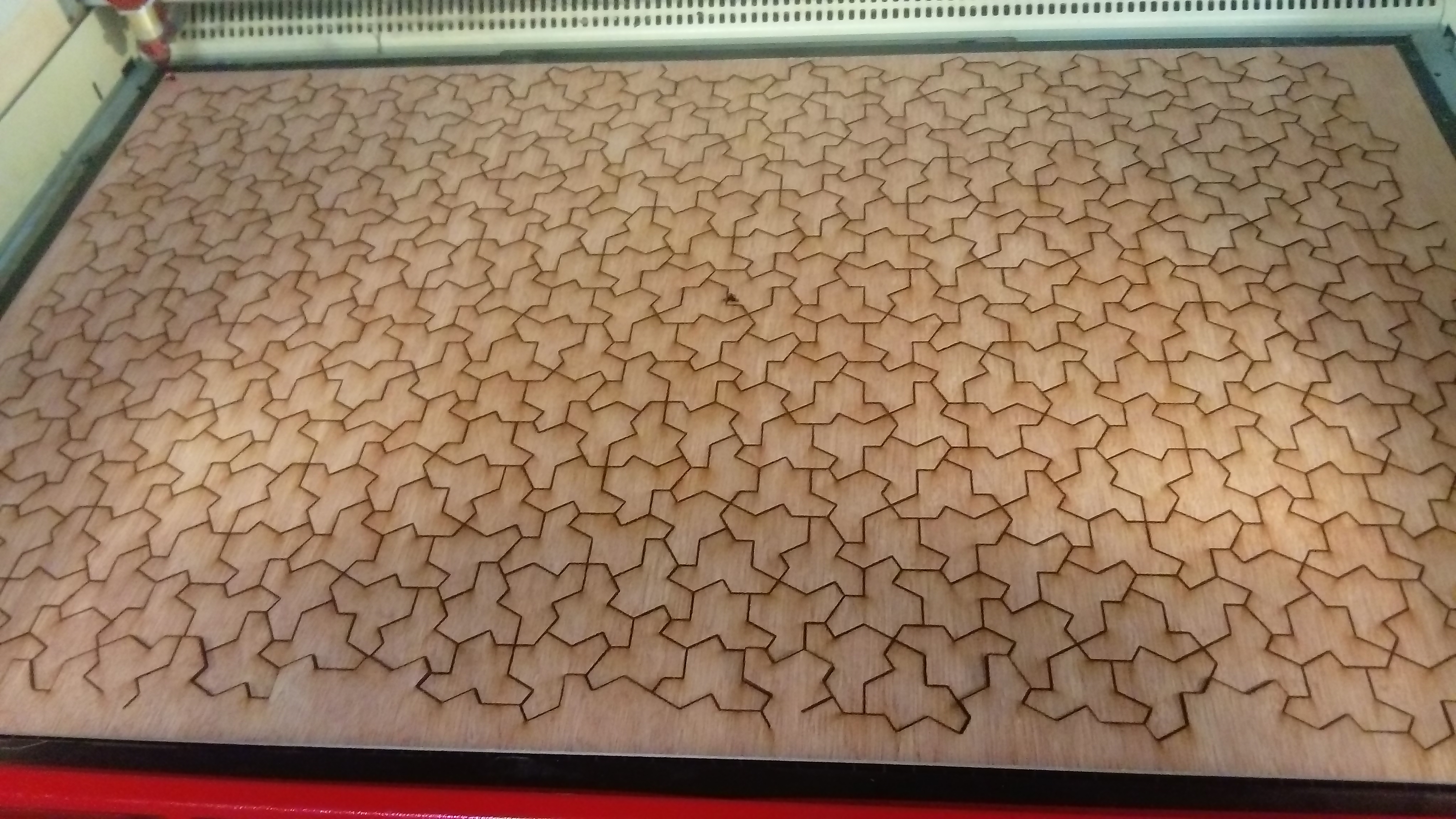
15 mai 2025 | Catégories: découpe laser, math | View CommentsEn janvier 2025, avec l'aide de David Renault, j'ai fait une nouvelle série de découpes lasers au fablab EirLab de l'ENSEIRB sur le thème des pavages par pentagones. Comme démontré par Michael Rao, il n'existe que 15 pavages pentagonaux possibles.
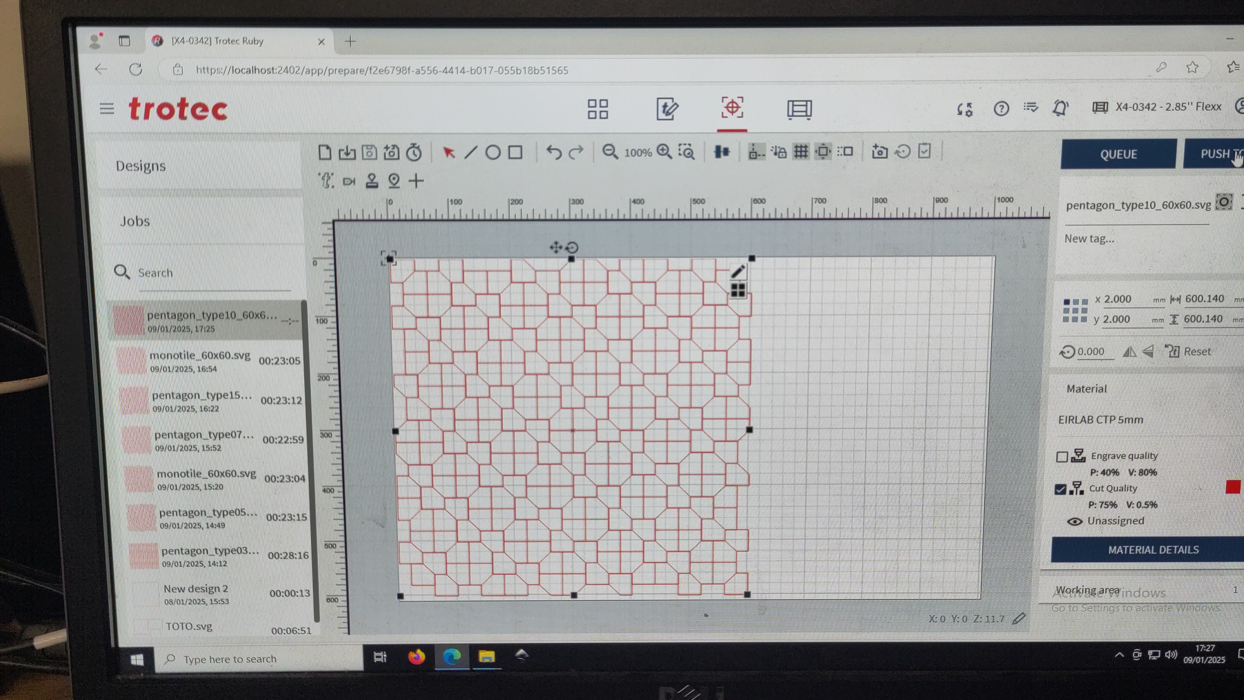
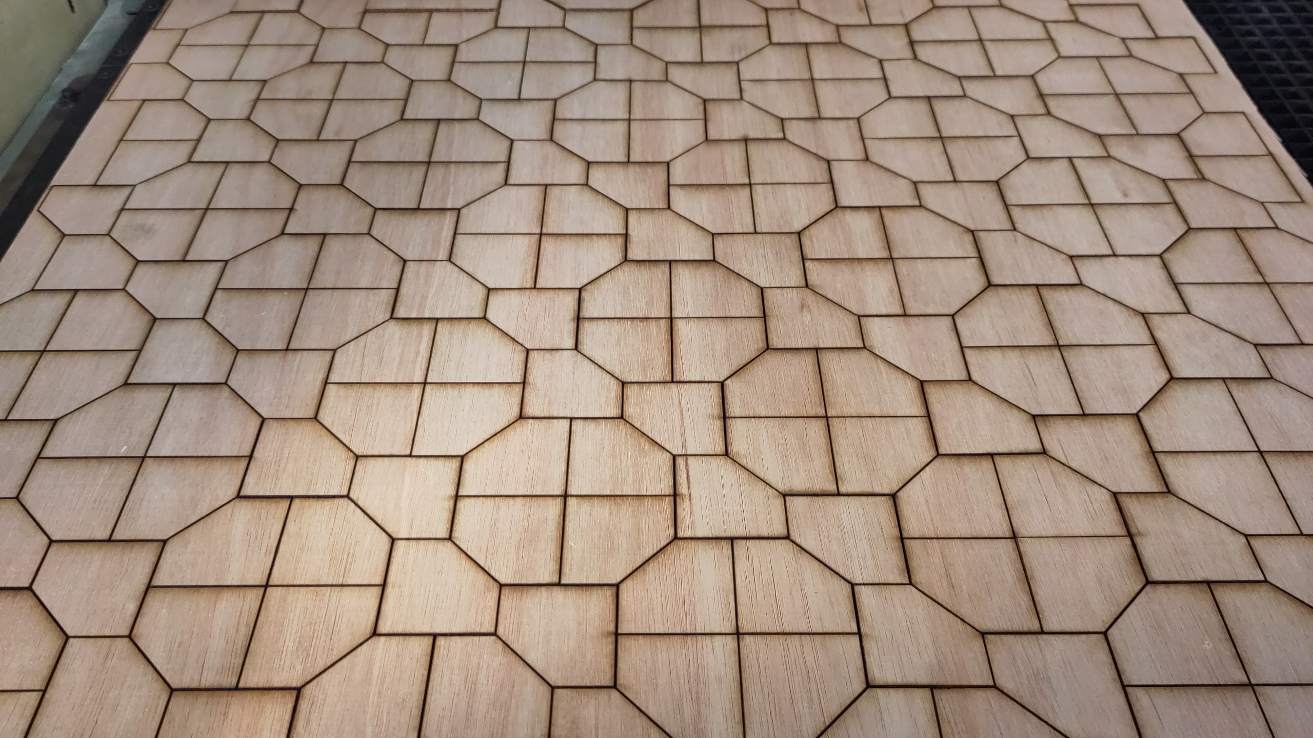
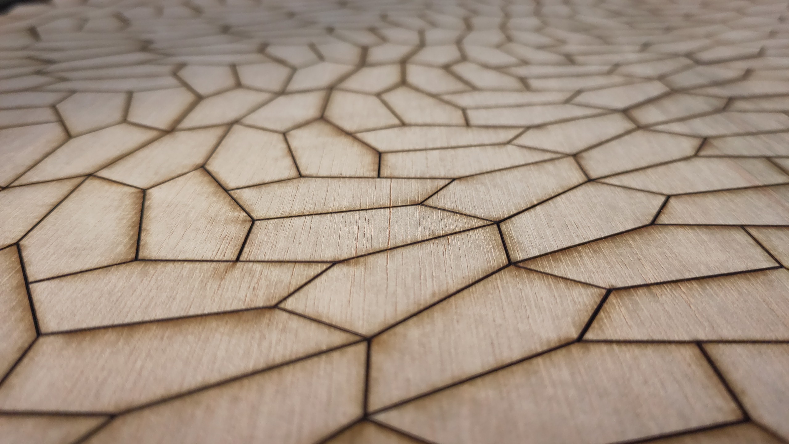
Voici quelques images de la découpe effectuée le 9 janvier 2025.
Un pentagone de type 7 découvert par Kershner en 1968:
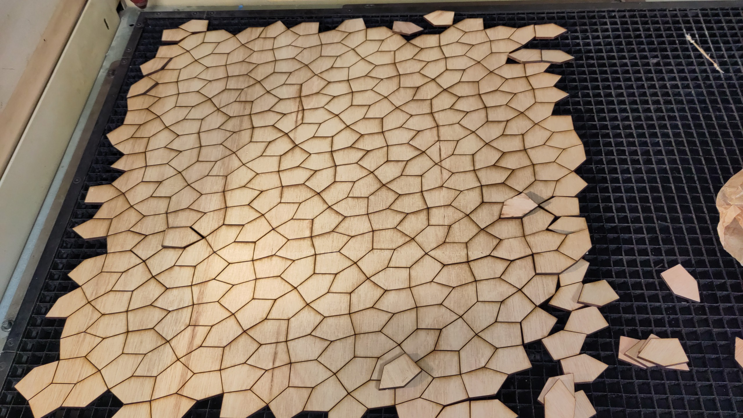
Un pentagone de type 10 découvert par James en 1975:
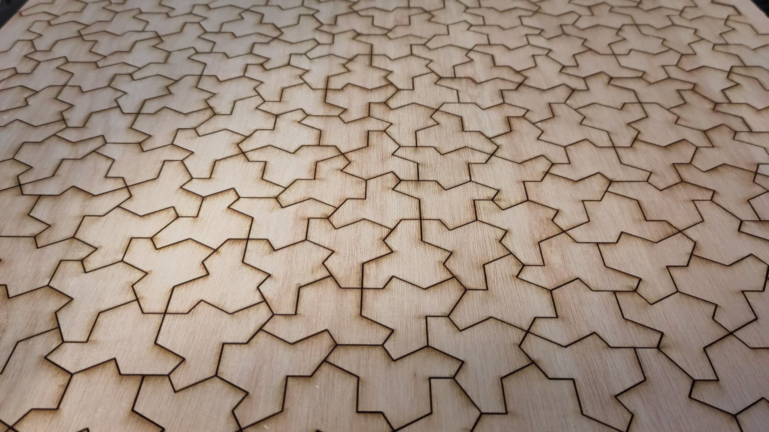
Le pentagone de type 15 découvert en 2015 par Jennifer McLoud-Mann, Casey Mann et David Von Derau, un étudiant de niveau licence en stage avec eux:
J'ai pu rencontrer Casey et Jennifer pour la première fois en 2017 à Montréal. Ils ont passé une année sabbatique à l'Université de Bordeaux en 2019-2020 via le programme Visiting Scholar de l'Université de Bordeaux, et cela a mené à une publication scientifique commune.
J'en ai aussi profité pour découper quelques tuiles chapeau apériodiques en plus:
Interventions dans les collèges et lycées en Gironde
Ces dernières années, sous l'invitation annuelle de Johanne Brengues, professeure au Lycée Kastler, j'ai développé un atelier sur la structure des flocons de neige et pavages apériodiques. Dans l'atelier d'une durée de 60 à 120 minutes, j'utilise des pièces en bois découpées au laser à l'ENSEIRB pour faire découvrir la science des pavages apériodiques et des quasicrystaux par la manipulation.
Pour l'année 2024-2025, j'ai soumis l'atelier suivant à l'Académie de Bordeaux dans le cadre de l'activité Des universitaires dans les classes.
Titre: Structure des flocons de neige et pavages apériodiques
Résumé: On dit que les flocons de neige sont tous différents. Pourquoi alors les branches d’un même flocon sont identiques? Dans cet exposé interactif, nous étudierons ces questions du point de vue des pavages du plan par des pièces de puzzle polygonales. Ces pièces se collent les unes aux autres comme le font en trois dimensions les molécules d’eau lors de la formation d’un flocon. En particulier, nous manipulerons des dizaines de copies d’un polygone à 13 côtés découvert en mars 2023. Les copies de ce polygone ont la propriété de paver le plan sans jamais se répéter. Nous utiliserons cet exemple pour discuter des pavages apériodiques du plan et de leurs propriétés. Public : tout niveau primaire + collège + lycée
J'ai été contacté par plusieurs collèges de la région pour faire cet atelier au printemps 2025:
- Collège Cassignol Bordeaux, 28 élèves de 3e, 7 janvier 2025
- Collège Jean Rostand, Casteljaloux, 3 classes de 6e, 16 janvier 2025
- Collège Olympe de Gouges, Vélines, 17 janvier 2025
- Village de maths, Collège Laure Gatet, Périgueux, 13 mars 2025
- Lycée Kastler, Talence, 15 mai 2025
- Collège Jean Zay, Cenon, 13 juin 2025
Les professeurs me disent que les pavages sont au programme du collège ce qui facilite les liens avec le sujet de l'atelier.
L'atelier en 2024-2025
Dans mes recherches, je m'intéresse à la combinatoire et à ses interactions avec les autres sciences. Par exemple, les atomes se combinent pour former des molécules stables en suivant des règles combinatoires simples. À l'état solide, les molécules peuvent se combiner pour former des structures ordonnées comme des crystaux ou même des flocons de neige.
La structure des flocons de neige est une science passionnante étudiée par Kenneth Libbrecht, professeur de physique au California Institute of Technology. Plusieurs questions naturelles peuvent-être posées par les élèves en voyant quelques images de flocons de neige:
- Pourquoi les flocons ont tous 6 branches?
- Pourquoi les branches d'un même flocon sont pareilles?
Après l'introduction sur la combinatoire et les flocons de neige, on passe à l'atelier. On divise la classe en petits groupes de 3 à 5 élèves. On attribue un atome (c'est-à-dire, plusieurs copies d'un même polygone) à chaque groupe. On demande aux élèves de trouver les molécules que l'atome peut créer en deux dimensions. On oriente les élèves à trouver des grandes molécules qui recouvrent des disques arbitrairement grand (on demande de recouvrir une feuille format A7, puis format A6, puis format A5, puis format A4).
Comme les pavages pentagonaux sont périodiques, nous démarrons l'atelier par l'exploration des pavages par l'un des 15 types de pentagones qui pavent le plan. Chaque groupe d'élèves se voit attribuer plusieurs copies d'une sorte de pentagones. Les élèves doivent explorer la combinatoire de la forme géométrique et faire des observations. Les découvertes des élèves sont publiées au tableau pendant l'atelier comme un article scientifique. Les résultats publiés peuvent être utilisés par les autres groupes à condition de les citer!
La notion d'apériodicité se transmet mieux après avoir compris la notion de pavages périodiques. La nouveauté pour mon atelier du printemps 2025 était de faire en sorte que les élèves découvrent d'abord des pavages périodiques non triviaux avant de considérer des pavages apériodiques. Cela permet de mieux expliquer la notion d'apériodicité.
Toutefois, avec une introduction de 15 à 20 minutes, l'atelier sur les pentagones nécessite presque la totalité du temps restant (30 minutes). Dans certains cas, un des groupes peut commencer l'étude de la pièce apériodique chapeau dans les 10 minutes restantes. Dans d'autres situations, je laisse un groupe choisir la pièce chapeau dès le début de l'atelier. Quand le temps le permet, on peut prévoir l'atelier en deux périodes de 60 minutes avec le même groupe. Cela permet d'explorer les pièces pentagonales périodiques, puis les pièces apériodiques tout en laissant du temps pour répondre aux questions des élèves.
Voici des fichiers qui rassemblent les images que j'utilise dans l'atelier sur les différents thèmes présentés.
Voici quelques liens pour en savoir plus:
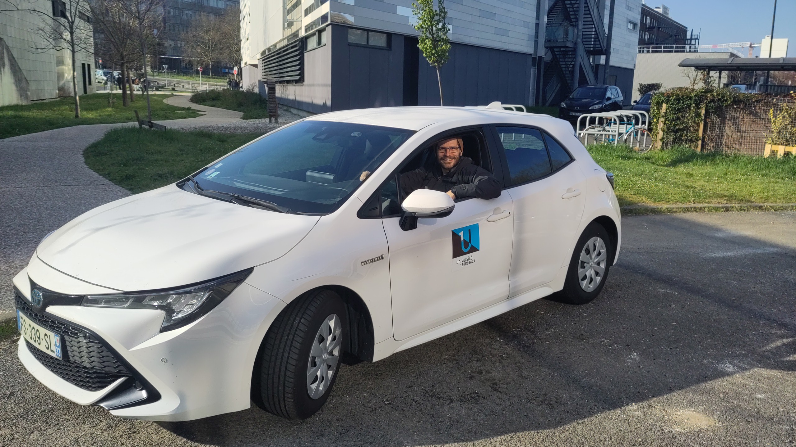
Pour les collèges et lycées en dehors de Bordeaux et difficilement accessible en transport en commun, je remercie l'Université de Bordeaux pour le prêt d'une voiture.
A do-it-yourself polygonal partition to construct Jeandel-Rao tilings
05 avril 2024 | Mise à jour: 07 février 2025 | Catégories: découpe laser, math | View CommentsIn 2015, Emmanuel Jeandel and Michael Rao discovered a very nice set of 11 Wang tiles which can be encoded geometrically into the following set of 11 geometrical shapes:
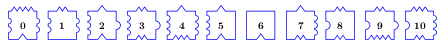
Jeandel and Rao proved that you may tile the plane with infinitely many translated copies of these tiles, but never periodically:
There is an easy way to construct Jeandel-Rao tilings from a well-chosen polygonal partition of the plane.
This is the polygonal partition:
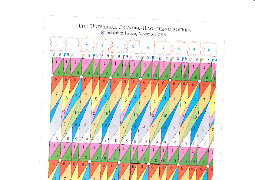
A lattice, represented below by the set of intersection of two perpendicular set of gridlines, is placed at a random position on top of the partition:
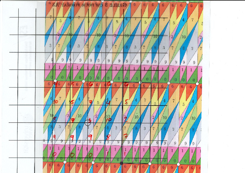
Each point of the lattice can be associated to an index from 0 to 10 according to which polygon of the partition it falls in. This defines a configuration of indices associated to each integer coordinate:
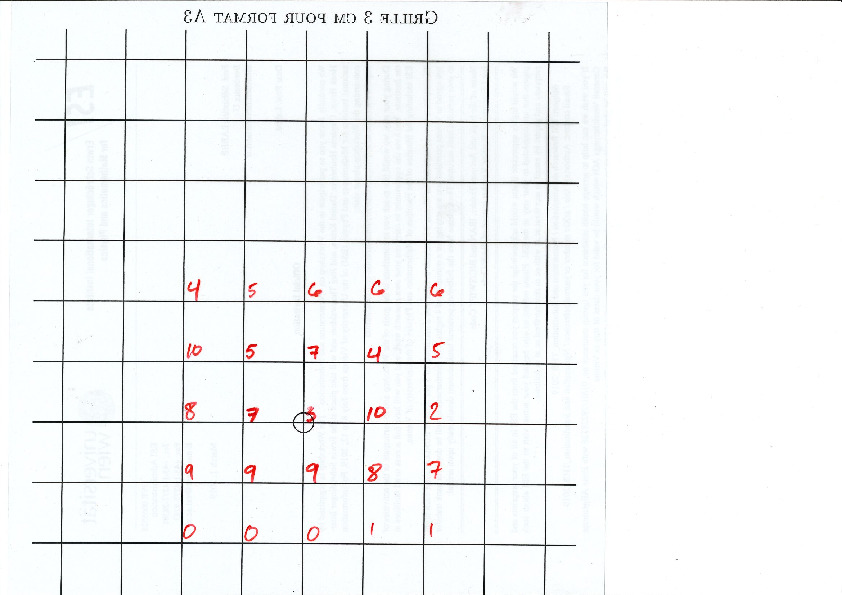
This procedure can be done all the way up to infinity. The chosen placement of the lattice defines a valid tiling of the plane with Jeandel-Rao tiles!

Since the size of the fundamental domain of the polygonal partition is irrational (width is golden mean, height is golden mean + 3, while the distance between two parallel gridlines is 1 unit), the generated configuration must be non-periodic.
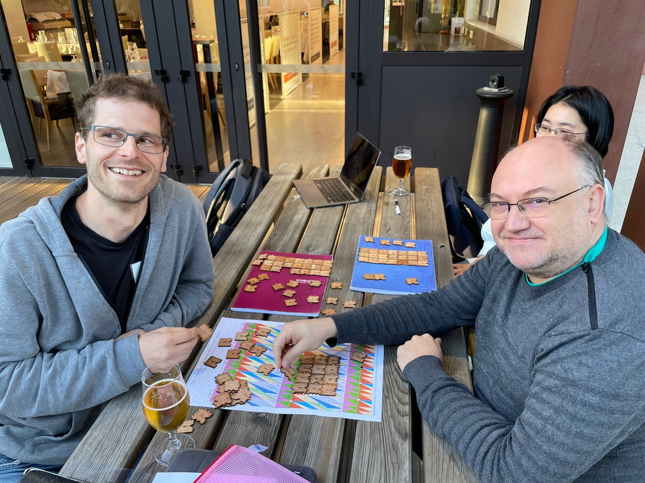
It was a pleasure for me to do illustrate this to Emmanuel Jeandel during the workshop Multidimensional symbolic dynamics and lattice models of quasicrystals at CIRM in April 2024 in Marseille.
Do it yourself
Here are the files allowing to reproduce this experiment:
- A 33 x 19 rectangular valid patch of 627 tiles to use to cut a 1 meter x 60 cm wooden flat sheet (in svg format for laser cutting, pieces should have a side length of exactly 3 cm after the operation)
- The polygonal partition to be printed on a A3 paper (1 unit = 3 cm)
- The lattice \(\mathbb{Z}^2\) represented by gridlines 3cm apart to be printed on A4 paper (1 unit = 3 cm)
- A one-page Jeandel-Rao tiling solver tutorial
- A two-page document gathering the tutorial + partition (A4 paper format)
Alternate files for laser cutting the tiles
I first cut those tiles in August 2018 before a conference in Durham with the help of David Renault. We made more of them in June 2019. Each time David does some changes to the file that I provide to him with InkScape. Here are three alternate files for laser cutting the tiles.
Frequency of tiles
The frequency of tiles in a Jeandel-Rao tilings is computed below from the relative area in the associated polygonal partition. Tile #2 is the least frequent (around 2.55%) while tile #7 is the most frequent (around 15%):
sage: from slabbe.arXiv_1903_06137 import jeandel_rao_wang_shift_partition
sage: P0 = jeandel_rao_wang_shift_partition()
sage: V = P0.volume()
sage: tile_frequency = {a:v/V for (a,v) in P0.volume_dict().items()}
sage: rows = [(a, tile_frequency[a], tile_frequency[a].n(digits=3)) for a in range(11)]
sage: table(rows, header_row=['tile', 'frequency', 'frequency (numerical approx)'])
  tile   frequency           frequency (numerical approx)
├──────┼───────────────────┼──────────────────────────────┤
  0      -1/22*phi + 2/11    0.108
  1      -1/22*phi + 2/11    0.108
  2      9/22*phi - 7/11     0.0255
  3      -1/22*phi + 2/11    0.108
  4      2/11*phi - 5/22     0.0669
  5      -5/11*phi + 9/11    0.0828
  6      -1/22*phi + 2/11    0.108
  7      -3/11*phi + 13/22   0.150
  8      2/11*phi - 5/22     0.0669
  9      -1/22*phi + 2/11    0.108
  10     2/11*phi - 5/22     0.0669
When I construct a bag of 50 tiles of the Jeandel-Rao tiles, I follow the above tile frequencies. It yields:
sage: [(tile_frequency[a]*52).n(digits=3) for a in range(11)]
[5.63, 5.63, 1.33, 5.63, 3.48, 4.30, 5.63, 7.78, 3.48, 5.63, 3.48]
sage: [round(a) for a in _]
[6, 6, 1, 6, 3, 4, 6, 8, 3, 6, 3]
sage: sum(_)
52
Discussion
The construction of valid tilings with Jeandel-Rao tiles from a polygonal partition is a generalization of a well-known phenomenon in one dimension, namely, the fact that Sturmian sequences of complexity \(n+1\) are coded by irrational rotations. For example, here is an easy way to construct Sturmian sequences using a partition of the line into two intervals of different lengths. Similarly as above, every point from a set of equidistanced points is coded by letter A or B according to which of the two intervals it falls in.
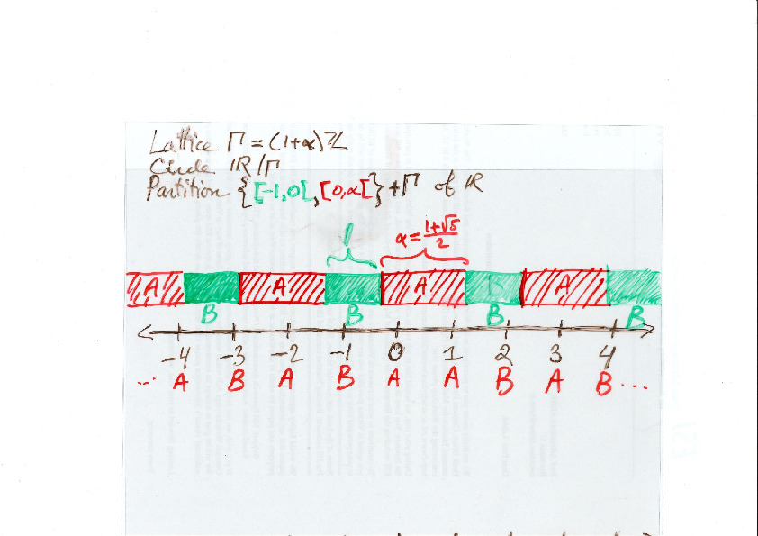
The question that one may ask is whether all Jeandel-Rao tilings can be constructed from such a starting point in the partition. For Sturmian sequences, the answer is yes and the starting point can be described using the Ostrowski numeration system and the continued fraction expansion of the slope defined from the ratio of frequencies of the letters in the sequence. In one dimension, the proof is thus based on the desubstitution of Sturmian sequences on the one hand, and the Rauzy induction of irrational rotations on the other hand.
The same approach can be performed for Jeandel-Rao tilings using 2-dimensional desubstitution of Wang tilings and 2-dimensional Rauzy induction of toral \(\mathbb{Z}^2\)-rotations. Surprisingly, the two totally different methods applied on two completely different objects lead to the same sequence of eventually periodic 2-dimensional substitutions. Thus, every Jeandel-Rao tiling that can be desubstituted indefinitely can be constructed from the coding of some starting point in the polygonal partition.
Unfortunately, not all Jeandel-Rao tilings can be desubstituted indefinitely because of the existence of a horizontal fault line breaking the substitutive structure. Some configuration have a biinfinite horizontal row of the same tile labeled 0 in them. This allows to slide the lower half of configuration along the fault line and the configuration remains valid. A conjecture is that the remaining configurations are rare (of probability zero according to any shift-invariant probability measure). More precisely, I believe that all of the problematic ones can be described by a pair of starting points on the bottom segment of the polygonal partition. During the sabbatical year of Casey Mann and Jennifer Mcloud-Mann in Bordeaux in 2019-2020, we tried hard to prove that conjecture without success. It seems to be a difficult problem. Instead we described the nonexpansive directions in Jeandel-Rao tilings which reminds of the behavior of Penrose tilings with respect to Conway worms, their resolutions and essential holes (annulus of tiles which can be completed uniquely outside of the annulus, but not inside).
Aperiodic tilings related to the Metallic mean
The structure of Penrose aperiodic tilings, Jeandel-Rao aperiodic tilings and the new aperiodic hat monotile are all related to the golden mean. Do all aperiodic tilings need to be related to the golden ratio? What other numbers can be achieved?
During the conference at CIRM, I presented my newest result split into two parts: for every positive integer \(n\), there exists an aperiodic set of \((n+3)^2\) Wang tiles whose tiling structure is associated to the \(n\)-th metallic mean number, that is, the positive root of the polynomial \(x^2-nx-1\). This new discovery extends the knowledge we have on aperiodic tilings beyond the omnipresent golden ratio. The talk was recorded on youtube and the written notes are available here.
Jean-René Chazottes et Marc Monticelli
During the conference at CIRM, I met Jean-René Chazottes and Marc Monticelli. They made me know about their interactive online books, the outreach mathemarium website and its online experiments. Also, the Open-Fabrik-Maths fablab in Nice, including some experiments involving aperiodic Wang tilings.
Découpe laser du chapeau, tuile apériodique découverte récemment
25 mai 2023 | Catégories: sage, slabbe spkg, math, découpe laser | View CommentsLe chapeau est une tuile apériodique découverte par David Smith, Joseph Samuel Myers, Craig S. Kaplan, et Chaim Goodman-Strauss le 20 mars 2023. Suite à un exposé donné le 26 mars au National Museum of Mathematics, la nouvelle s'est vite répandue. En effet, cette découverte a été mentionnée les jours suivants dans des blogues puis dans Le New York Times le 28 mars, Le Monde le 29 mars, puis The Guardian et QuantaMagazine le 4 avril. Un vidéo de 20 minutes, réalisé par Passe-Science et publié début le 3 mai, explique le résultat et son contexte.
Déjà des articles proposant des résultats plus approfondis sur la tuile par des experts du domaine sont parus sur arXiv en mai 2023. Ils interprêtent les pavages comme des coupes et projection de réseaux de dimension supérieure. Le deuxième propose même une partition de la fenêtre de l'espace interne, un peu comme pour les pavages de Jeandel-Rao, à la différence qu'ici la partition a des bords fractales ce qui est pour moi une grande surprise.
Comme je faisais une intervention dans l'école de mon garçon à Bègles le 3 mai et au Lycée Kastler de Talence le 4 mai, j'ai réalisé un projet de découpe laser sur la tuile apériodique afin de partager cette récente découverte.
La première question était de construire un pavage d'un rectangle assez grand avec la pièce apériodique. Pour ce faire, j'ai ajouté un nouveau module dans mon package optionel au logiciel SageMath.
Le module réalise une réduction à une instance du problème de la couverture universelle, qui peut être résolu dans SageMath en utilisant l'algorithme des liens dansants de Donald Knuth, les solveurs SAT ou les programmes d'optimisation linéaire (solveur MILP). Le code utilise le système de coordonnées défini dans le fichier validate/kitegrid.pdf qui se trouve dans le code source associé à l'article.
Voici un exemple de construction d'un pavage avec la tuile apériodique. Le calcul est fait dans le logiciel SageMath muni de la version de développement de mon package optionnel slabbe qui peut être installé avec la commande sage -pip install slabbe. Ici, j'utilise le solveur SAT Glucose, développé au LaBRI. On peut installer glucose dans SageMath avec la commande sage -i glucose.
sage: from slabbe.aperiodic_monotile import MonotileSolver
sage: s = MonotileSolver(16, 17)
sage: G = s.draw_one_solution(solver='glucose')
sage: G.save('solution_16x17.png')
sage: G
Dans la manière de résoudre la question ci-haut, le problème est représenté par un problème de couverture exacte qui consiste à recouvrir exactement les entiers de 1 à n avec des sous-ensembles choisis dans une liste de sous-ensembles déterminés. Ici, on représente l'espace à recouvrir de manière discrète en comptant 6 points du plan par hexagone (un point pour chaque kite contenu dans un hexagone). Rappelons que la pièce Chapeau qui nous intéresse est formée d'une union d'exactement 8 de ces kites.
sage: s.plot_domain()
Ensuite, on construit une matrice de 0 et de 1 avec autant de colonnes que de points ci-haut (16 * 17 * 2 * 6 = 3264) et autant de lignes qu'il y a de copies isométriques de la pièce intersectant le domaine. Pour chaque copie de la pièce, une ligne dans la matrice contient des 1 exactement dans les colonnes associées aux kites occupés par la pièce.
sage: s.the_dlx_solver()
Dancing links solver for 3264 columns and 7116 rows
Le calcul ci-haut qui a construit la matrice (sparse) indique qu'il y a 7116 copies isométriques de la pièce qui intersectent (complètement ou partiellement) le domaine. Quand on voudra dessiner une solution, on ignorera les pièces incomplètes.
On peut maintenant résoudre le problème.
sage: s = MonotileSolver(8,8)
sage: %time L = s.one_solution()   # l'algo des liens dansants de Knuth est utilisé par défaut
CPU times: user 798 ms, sys: 32.2 ms, total: 830 ms
Wall time: 1min 20s
Le contenu d'une solution est une liste de nombres indiquant les lignes de la matrice de 0/1 à considérer pour former une solution. C'est-à-dire que la sous-matrice restreinte aux lignes données comporte exactement un 1 dans chaque colonne:
sage: L
[81,
 85,
 125,
 128,
 ...
 1772,
 1783,
 1794,
 1815]
Ici, il se trouve que les solveurs SAT sont plus efficaces que l'algo des liens dansants pour trouver une solution:
sage: %time L = s.one_solution(solver='glucose')
CPU times: user 326 ms, sys: 16.1 ms, total: 342 ms
Wall time: 526 ms
sage: %time L = s.one_solution(solver='kissat')
CPU times: user 335 ms, sys: 3.64 ms, total: 339 ms
Wall time: 461 ms
En effet, Glucose se comporte plutôt bien pour résoudre des problèmes de pavages du plan lorsqu'il existe une solution. Mais lorsqu'il n'y a pas de solution, l'algo des liens dansants de Knuth est parfois mieux. Aussi, l'algo des liens dansants de Knuth est très efficace pour énumérer toutes les solutions.
Le solveur Kissat a été ajouté dans SageMath par moi-même comme package optionnel cette année suite à une discussion avec Laurent Simon au café du LaBRI. On peut installer le solveur kissat dans SageMath avec la commande sage -i kissat.
Ici on extrait le contour des pièces d'une solution (tel que chaque arête est dessinée une seule fois afin d'éviter que la découpeuse laser passe deux fois par chaque arête ce qui peut endommager ou brûler le bord des pièces en bois) et on crée un fichier pdf ou svg. Je choisis une taille de 16 double-hexagones horizontalement et 17 verticalement, car cela crée un fichier qui correspond à une taille de 1m x 60cm. C'est la taille de la découpeuse laser à notre disposition:
sage: s = MonotileSolver(16, 17)
sage: tikz = s.one_solution_tikz(solver='glucose')
sage: tikz.pdf('solution_16x17.pdf')
sage: tikz.svg('solution_16x17.svg')     # or
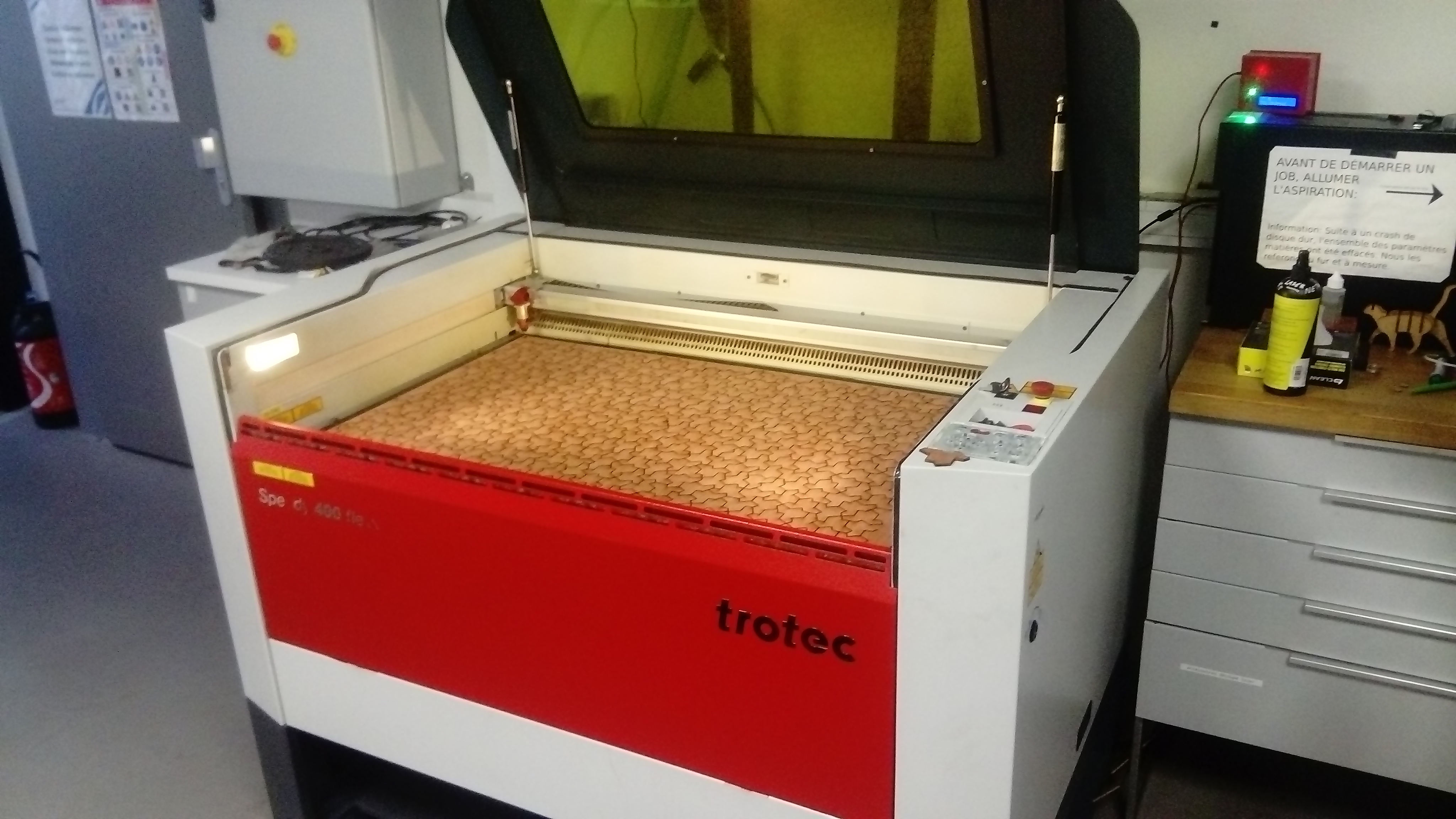
Avec l'aide de David Renault, mon collègue du LaBRI qui enseigne à l'ENSEIRB et qui m'a déjà accompagné dans la réalisation de projets de découpe laser, nous avons découpé le fichier ci-haut le jeudi 27 avril au EirLab, l'atelier de fabrication numérique (FabLab) de l'ENSEIRB-MATMECA:
Comme toujours, il faut quelque peu modifier le fichier svg dans Inkscape avant de lancer la découpe laser. Voici le fichier modifié juste avant la découpe.
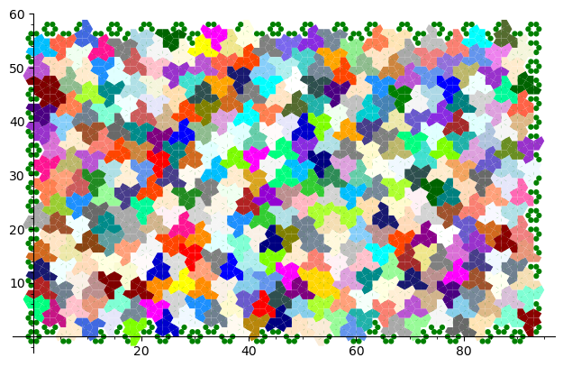
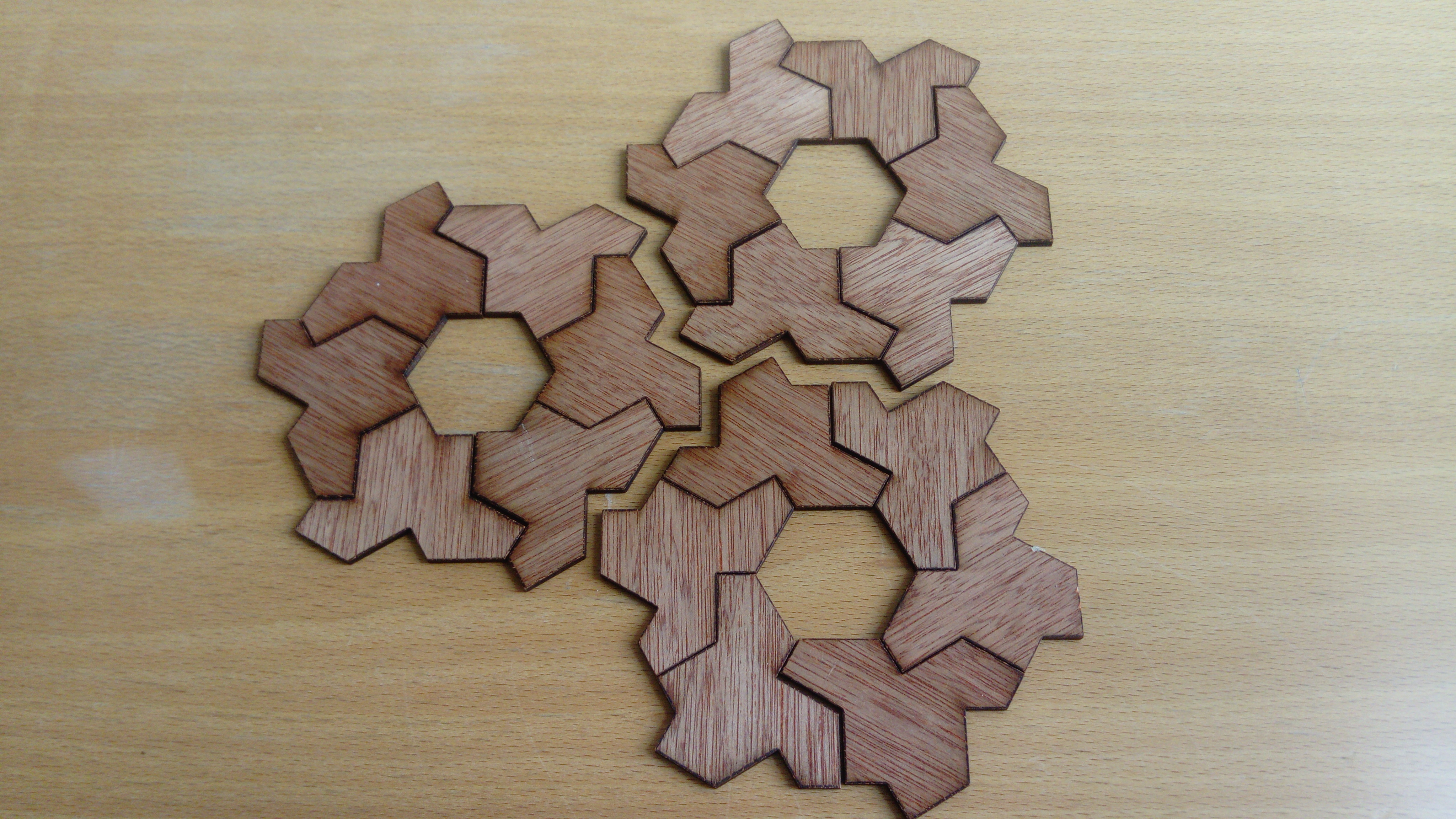
Maintenant, on peut s'amuser avec les pièces:
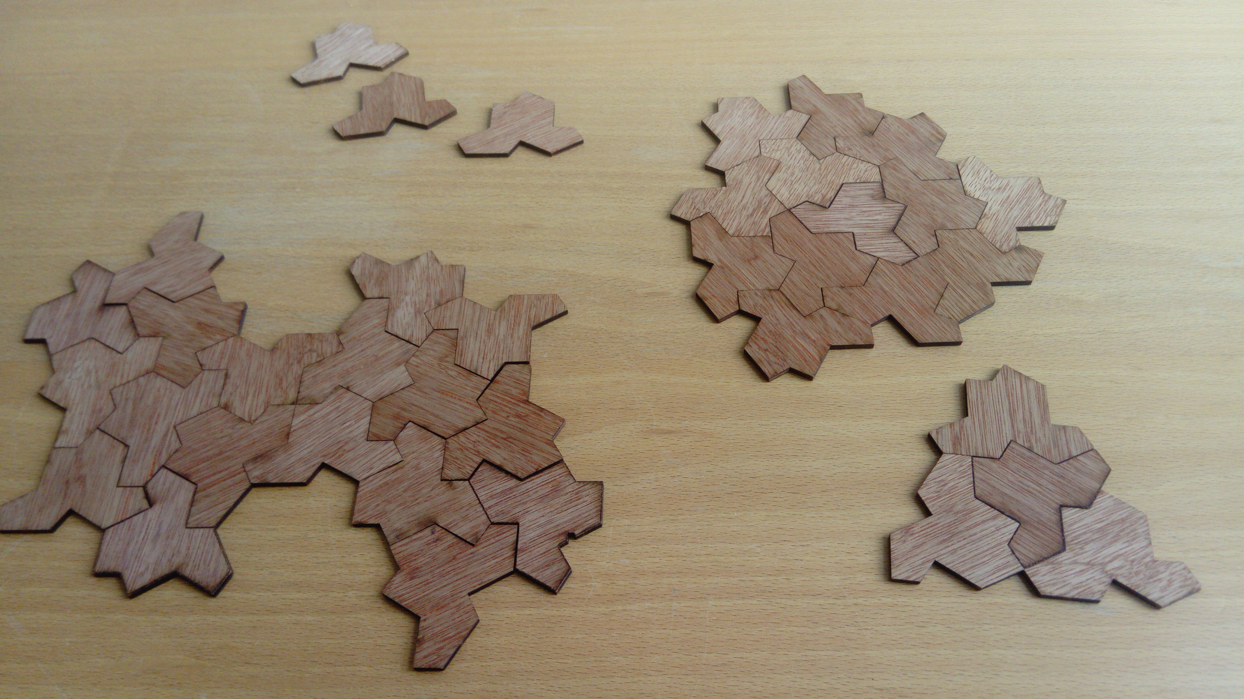
Avec mes garçons, nous avons trouvé une forme intéressante qui recouvre le plan périodiquement à l'exception d'un trou hexagonal. Il se trouve que la même forme peut-être créée de deux façons différentes: sur l'image ci-bas la forme à droite est la globalement la même, mais elle n'est pas obtenue de la même façon que celle en haut à gauche. Pourtant, toutes deux ont le même contour extérieur et le même trou hexagonal.
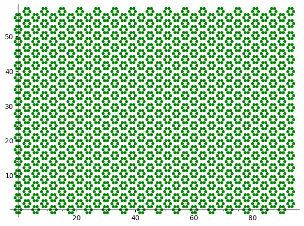
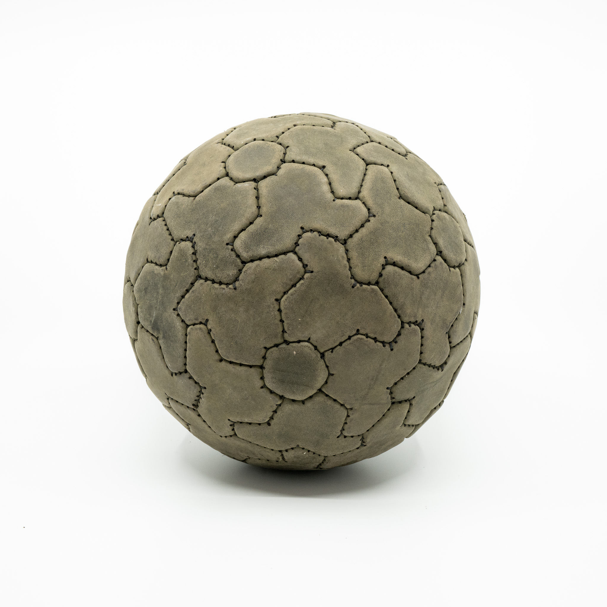
Cette observation, déjà faite par d'autres, a mené au recouvrement d'une sphère avec la pièce et un trou pentagonal:
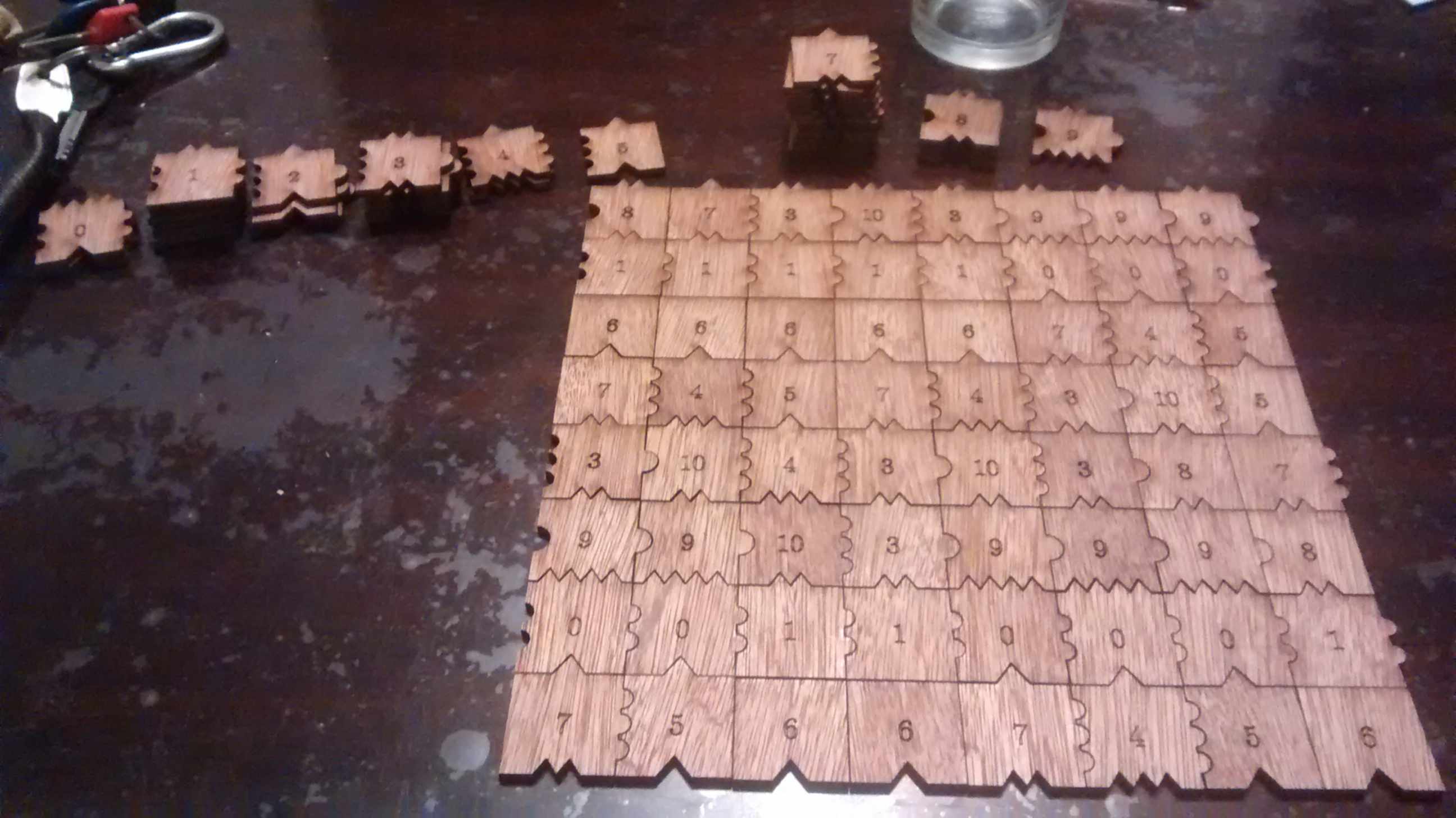
Wooden laser-cut Jeandel-Rao tiles
07 septembre 2018 | Catégories: sage, slabbe spkg, math, découpe laser | View CommentsI have been working on Jeandel-Rao tiles lately.
Before the conference Model Sets and Aperiodic Order held in Durham UK (Sep 3-7 2018), I thought it would be a good idea to bring some real tiles at the conference. So I first decided of some conventions to represent the above tiles as topologically closed disk basically using the representation of integers in base 1:
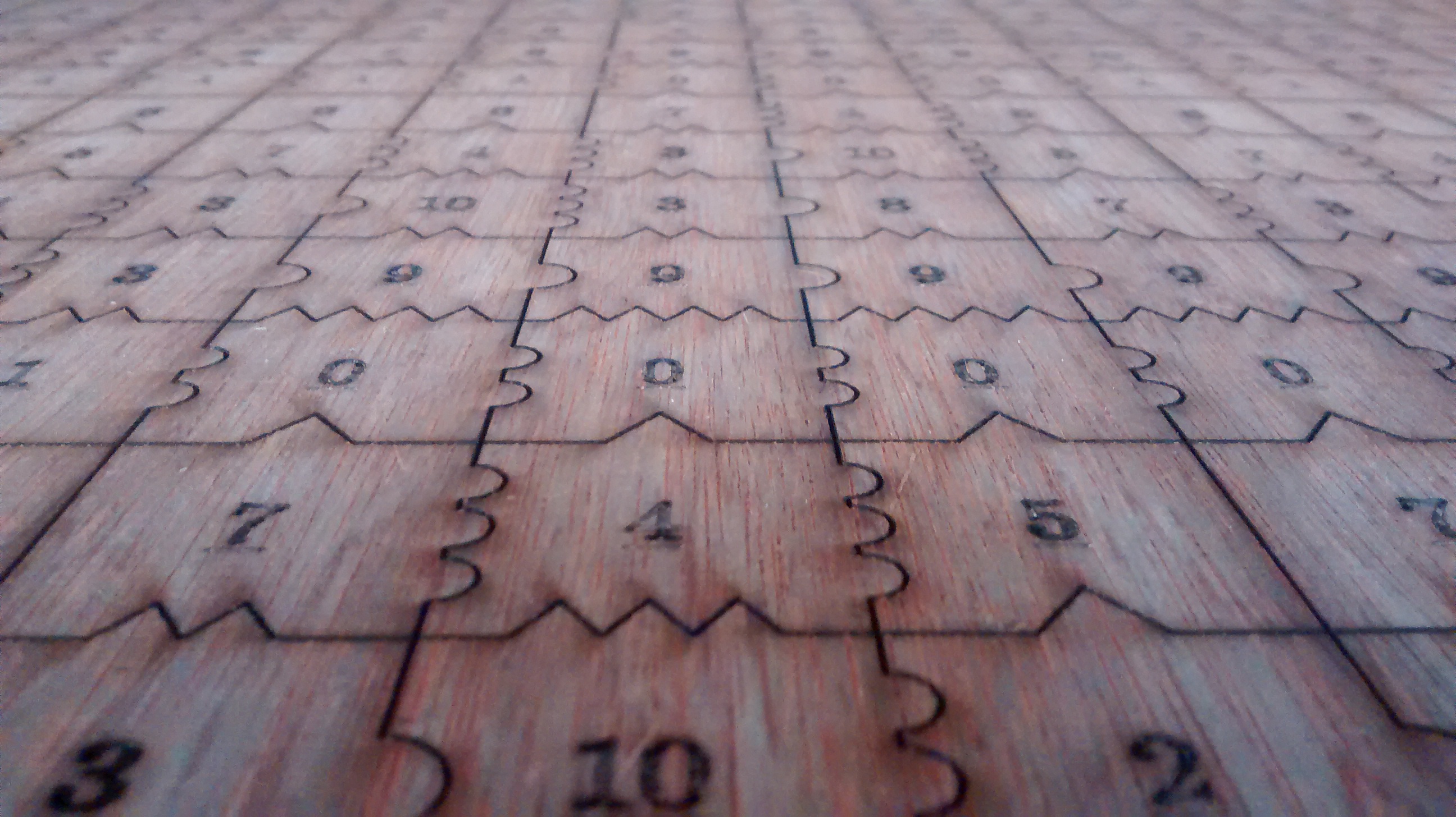
With these shapes, I created a 33 x 19 patch. With 3cm on each side, the patch takes 99cm x 57cm just within the capacity of the laser cut machine (1m x 60 cm):
With the help of David Renault from LaBRI, we went at Coh@bit, the FabLab of Bordeaux University and we laser cut two 3mm thick plywood for a total of 1282 Wang tiles. This is the result:
One may recreate the 33 x 19 tiling as follows (note that I am using Cartesian-like coordinates, so the first list data[0] actually is the first column from bottom to top):
sage: data = [[10, 4, 6, 1, 3, 3, 7, 0, 9, 7, 2, 6, 1, 3, 8, 7, 0, 9, 7],
....:  [4, 5, 6, 1, 8, 10, 4, 0, 9, 3, 8, 7, 0, 9, 7, 5, 0, 9, 3],
....:  [3, 7, 6, 1, 7, 2, 5, 0, 9, 8, 7, 5, 0, 9, 3, 7, 0, 9, 10],
....:  [10, 4, 6, 1, 3, 8, 7, 0, 9, 7, 5, 6, 1, 8, 10, 4, 0, 9, 3],
....:  [2, 5, 6, 1, 8, 7, 5, 0, 9, 3, 7, 6, 1, 7, 2, 5, 0, 9, 8],
....:  [8, 7, 6, 1, 7, 5, 6, 1, 8, 10, 4, 6, 1, 3, 8, 7, 0, 9, 7],
....:  [7, 5, 6, 1, 3, 7, 6, 1, 7, 2, 5, 6, 1, 8, 7, 5, 0, 9, 3],
....:  [3, 7, 6, 1, 10, 4, 6, 1, 3, 8, 7, 6, 1, 7, 5, 6, 1, 8, 10],
....:  [10, 4, 6, 1, 3, 3, 7, 0, 9, 7, 5, 6, 1, 3, 7, 6, 1, 7, 2],
....:  [2, 5, 6, 1, 8, 10, 4, 0, 9, 3, 7, 6, 1, 10, 4, 6, 1, 3, 8],
....:  [8, 7, 6, 1, 7, 5, 5, 0, 9, 10, 4, 6, 1, 3, 3, 7, 0, 9, 7],
....:  [7, 5, 6, 1, 3, 7, 6, 1, 10, 4, 5, 6, 1, 8, 10, 4, 0, 9, 3],
....:  [3, 7, 6, 1, 10, 4, 6, 1, 3, 3, 7, 6, 1, 7, 2, 5, 0, 9, 8],
....:  [10, 4, 6, 1, 3, 3, 7, 0, 9, 10, 4, 6, 1, 3, 8, 7, 0, 9, 7],
....:  [4, 5, 6, 1, 8, 10, 4, 0, 9, 3, 3, 7, 0, 9, 7, 5, 0, 9, 3],
....:  [3, 7, 6, 1, 7, 2, 5, 0, 9, 8, 10, 4, 0, 9, 3, 7, 0, 9, 10],
....:  [10, 4, 6, 1, 3, 8, 7, 0, 9, 7, 5, 5, 0, 9, 10, 4, 0, 9, 3],
....:  [2, 5, 6, 1, 8, 7, 5, 0, 9, 3, 7, 6, 1, 10, 4, 5, 0, 9, 8],
....:  [8, 7, 6, 1, 7, 5, 6, 1, 8, 10, 4, 6, 1, 3, 3, 7, 0, 9, 7],
....:  [7, 5, 6, 1, 3, 7, 6, 1, 7, 2, 5, 6, 1, 8, 10, 4, 0, 9, 3],
....:  [3, 7, 6, 1, 10, 4, 6, 1, 3, 8, 7, 6, 1, 7, 2, 5, 0, 9, 8],
....:  [10, 4, 6, 1, 3, 3, 7, 0, 9, 7, 2, 6, 1, 3, 8, 7, 0, 9, 7],
....:  [4, 5, 6, 1, 8, 10, 4, 0, 9, 3, 8, 7, 0, 9, 7, 5, 0, 9, 3],
....:  [3, 7, 6, 1, 7, 2, 5, 0, 9, 8, 7, 5, 0, 9, 3, 7, 0, 9, 10],
....:  [10, 4, 6, 1, 3, 8, 7, 0, 9, 7, 5, 6, 1, 8, 10, 4, 0, 9, 3],
....:  [3, 3, 7, 0, 9, 7, 5, 0, 9, 3, 7, 6, 1, 7, 2, 5, 0, 9, 8],
....:  [8, 10, 4, 0, 9, 3, 7, 0, 9, 10, 4, 6, 1, 3, 8, 7, 0, 9, 7],
....:  [7, 5, 5, 0, 9, 10, 4, 0, 9, 3, 3, 7, 0, 9, 7, 5, 0, 9, 3],
....:  [3, 7, 6, 1, 10, 4, 5, 0, 9, 8, 10, 4, 0, 9, 3, 7, 0, 9, 10],
....:  [10, 4, 6, 1, 3, 3, 7, 0, 9, 7, 5, 5, 0, 9, 10, 4, 0, 9, 3],
....:  [2, 5, 6, 1, 8, 10, 4, 0, 9, 3, 7, 6, 1, 10, 4, 5, 0, 9, 8],
....:  [8, 7, 6, 1, 7, 5, 5, 0, 9, 10, 4, 6, 1, 3, 3, 7, 0, 9, 7],
....:  [7, 5, 6, 1, 3, 7, 6, 1, 10, 4, 5, 6, 1, 8, 10, 4, 0, 9, 3]]
The above patch have been chosen among 1000 other randomly generated as the closest to the asymptotic frequencies of the tiles in Jeandel-Rao tilings (or at least in the minimal subshift that I describe in the preprint):
sage: from collections import Counter
sage: c = Counter(flatten(data))
sage: tile_count = [c[i] for i in range(11)]
The asymptotic frequencies:
sage: phi = golden_ratio.n()
sage: Linv = [2*phi + 6, 2*phi + 6, 18*phi + 10, 2*phi + 6, 8*phi + 2,
....:      5*phi + 4, 2*phi + 6, 12/5*phi + 14/5, 8*phi + 2,
....:      2*phi + 6, 8*phi + 2]
sage: perfect_proportions = vector([1/a for a in Linv])
Comparison of the number of tiles of each type with the expected frequency:
sage: header_row = ['tile id', 'Asymptotic frequency', 'Expected nb of copies',
....:               'Nb copies in the 33x19 patch']
sage: columns = [range(11), perfect_proportions, vector(perfect_proportions)*33*19, tile_count]
sage: table(columns=columns, header_row=header_row)
  tile id   Asymptotic frequency   Expected nb of copies   Nb copies in the 33x19 patch
+---------+----------------------+-----------------------+------------------------------+
  0         0.108271182329550      67.8860313206280        67
  1         0.108271182329550      67.8860313206280        65
  2         0.0255593590340479     16.0257181143480        16
  3         0.108271182329550      67.8860313206280        71
  4         0.0669152706817991     41.9558747174880        42
  5         0.0827118232955023     51.8603132062800        51
  6         0.108271182329550      67.8860313206280        65
  7         0.149627093977301      93.8161879237680        95
  8         0.0669152706817991     41.9558747174880        44
  9         0.108271182329550      67.8860313206280        67
  10        0.0669152706817991     41.9558747174880        44
I brought the \(33\times19=641\) tiles at the conference and offered to the first 7 persons to find a \(7\times 7\) tiling the opportunity to keep the 49 tiles they used. 49 is a good number since the frequency of the lowest tile (with id 2) is about 2% which allows to have at least one copy of each tile in a subset of 49 tiles allowing a solution.
A natural question to ask is how many such \(7\times 7\) tilings does there exist? With ticket #25125 that was merged in Sage 8.3 this Spring, it is possible to enumerate and count solutions in parallel with Knuth dancing links algorithm. After the installation of the Sage Optional package slabbe (sage -pip install slabbe), one may compute that there are 152244 solutions.
sage: from slabbe import WangTileSet
sage: tiles = [(2,4,2,1), (2,2,2,0), (1,1,3,1), (1,2,3,2), (3,1,3,3),
....: (0,1,3,1), (0,0,0,1), (3,1,0,2), (0,2,1,2), (1,2,1,4), (3,3,1,2)]
sage: T0 = WangTileSet(tiles)
sage: T0_solver = T0.solver(7,7)
sage: %time T0_solver.number_of_solutions(ncpus=8)
CPU times: user 16 ms, sys: 82.3 ms, total: 98.3 ms
Wall time: 388 ms
152244
One may also get the list of all solutions and print one of them:
sage: %time L = T0_solver.all_solutions(); print(len(L))
152244
CPU times: user 6.46 s, sys: 344 ms, total: 6.8 s
Wall time: 6.82 s
sage: L[0]
A wang tiling of a 7 x 7 rectangle
sage: L[0].table()  # warning: the output is in Cartesian-like coordinates
[[1, 8, 10, 4, 5, 0, 9],
 [1, 7, 2, 5, 6, 1, 8],
 [1, 3, 8, 7, 6, 1, 7],
 [0, 9, 7, 5, 6, 1, 3],
 [0, 9, 3, 7, 6, 1, 8],
 [1, 8, 10, 4, 6, 1, 7],
 [1, 7, 2, 2, 6, 1, 3]]
This is the number of distinct sets of 49 tiles which admits a 7x7 solution:
sage: from collections import Counter
sage: def count_tiles(tiling):
....:     C = Counter(flatten(tiling.table()))
....:     return tuple(C.get(a,0) for a in range(11))
sage: Lfreq = map(count_tiles, L)
sage: Lfreq_count = Counter(Lfreq)
sage: len(Lfreq_count)
83258
Number of other solutions with the same set of 49 tiles:
sage: Counter(Lfreq_count.values())
Counter({1: 49076, 2: 19849, 3: 6313, 4: 3664, 6: 1410, 5: 1341, 7: 705, 8:
293, 9: 159, 14: 116, 10: 104, 12: 97, 18: 44, 11: 26, 15: 24, 13: 10, 17: 8,
22: 6, 32: 6, 16: 3, 28: 2, 19: 1, 21: 1})
How the number of \(k\times k\)-solutions grows for k from 0 to 9:
sage: [T0.solver(k,k).number_of_solutions() for k in range(10)]
[0, 11, 85, 444, 1723, 9172, 50638, 152244, 262019, 1641695]
Unfortunately, most of those \(k\times k\)-solutions are not extendable to a tiling of the whole plane. Indeed the number of \(k\times k\) patches in the language of the minimal aperiodic subshift that I am able to describe and which is a proper subset of Jeandel-Rao tilings seems, according to some heuristic, to be something like:
[1, 11, 49, 108, 184, 268, 367, 483]
I do not share my (ugly) code for this computation yet, as I will rather share clean code soon when times come. So among the 152244 about only 483 (0.32%) of them are prolongable into a uniformly recurrent tiling of the plane.
Propulsé par Blogofile
S'abonner au Flux RSS
et aux Commentaires.

This work by Sébastien Labbé is licensed under a Creative Commons Attribution-ShareAlike 4.0 International License.