On the bifurcation diagram proposed by Jang and Robinson
06 mai 2025 | Catégories: sage, math | View CommentsIn this blog post, we present a few remarks on the "bifurcation diagram" proposed by Jang and Robinson in [1] to describe the tilings associated to a set of 24 Wang tiles encoding Penrose tilings.
[1] Hyeeun Jang, E. Arthur Robinson Jr, Directional Expansiveness for Rd-Actions and for Penrose Tilings, arxiv:2504.10838
In particular, I believe that something is wrong in what the authors call the "bifurcation diagram" shown in Figure 10. But, as we illustrate below, it can be fixed easily by permuting some of the labels of the partition.
I saw Jang and Robinsion's bifurcation diagram for the first time during the talk "Remembering Shunji Ito" made by Robinson during the online conference dedicated to the memory of Shunji Ito on December 14, 2021. At that time, I was working on the family of metallic mean Wang tiles. This is why the bifurcation diagram shown by Robinson and extracted from Jang's PhD thesis got my attention right away, because it was looking very much like the Markov partition associated to the Ammann set of 16 Wang tiles, the first member of the family of metallic mean Wang tiles. As we illustrate below, Jang and Robinson's bifurcation diagram is a refinement of the Markov partition associated the Ammann set of 16 Wang tiles. This means that the 16 tiles Ammann Wang shift is a factor of the 24 tiles Penrose Wang shift. Also most probably the bifurcation diagram is a Markov Partition for the same associated toral ℤ2-action. But this needs a proof.
The content of this blog post is also available as a Jupyter notebook that can be viewed and downloaded from the nbviewer.
Dependencies
The computations made here depend on the modules WangTileSet, WangTiling, PolyhedronPartition, PolyhedronExchangeTransformation, PETsCoding implemented in the SageMath optional package slabbe over the last years in order to describe and study the Jeandel-Rao aperiodic tilings and the family of metallic mean Wang tiles.
Note that the package slabbe can be installed by running !pip install slabbe directly in SageMath:
sage: # !pip install slabbe # uncomment and execute this line to install slabbe package
Here are the version of the packages used in this post:
sage: import importlib
sage: importlib.metadata.version("slabbe")
'0.8.0'
sage: version()
'SageMath version 10.5.beta6, Release Date: 2024-09-29'
Jang-Robinson encoding of the Penrose 24 Wang tiles
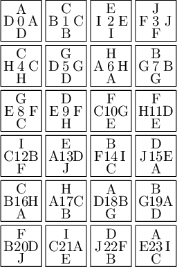
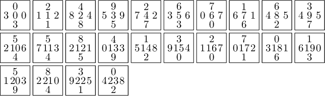
We encode the 24 Wang tiles proposed by Jang and Robinson (Figure 9 of [1]) using alphabet {A, B, C, D, E, F, G, H, I, J} for the shapes:
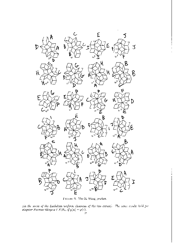
We define the 24 Wang tiles in SageMath:
sage: from slabbe import WangTileSet, WangTiling
sage: tiles = ["AADD", "CCBB", "EEII", "JJFF",
....:          "CCHH", "GGDD", "HHAA", "BBGG",
....:          "FGEC", "FDEH", "GFCE", "DFHE",
....:          "BICF", "DEAJ", "IBFC", "EDJA",
....:          "HCBA", "CHAB", "BADG", "ABGD",
....:          "DFBJ", "AICE", "FDJB", "IAEC"]
sage: T0 = WangTileSet([tuple(str(a) for a in tile) for tile in tiles])
sage: T0
Wang tile set of cardinality 24
sage: T0.tikz(ncolumns=4)
Constructing Jang-Robinson Bifurcation diagram as a polygonal partition
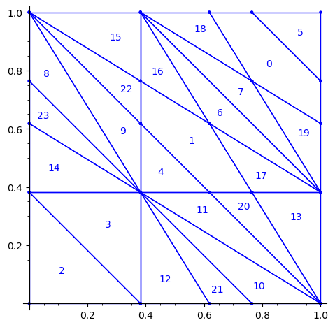
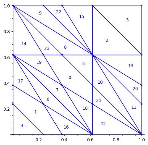
Below is a reproduction of Jang-Robinson bifurcation diagram shown in Figure 10 from arxiv:2504.10838
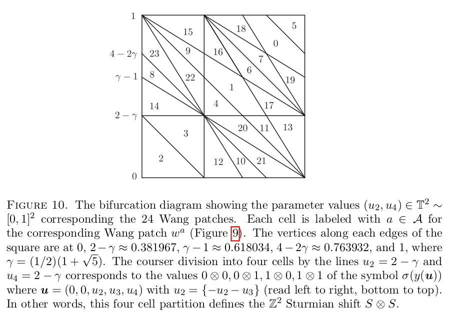
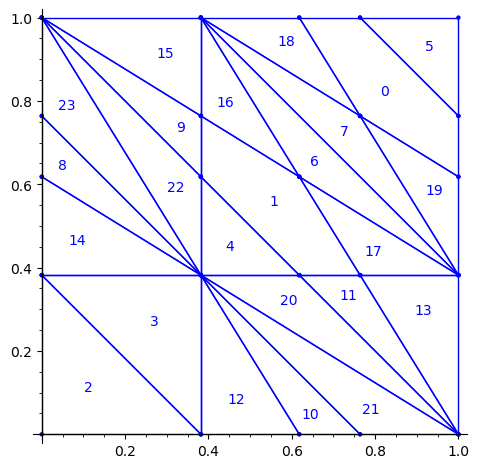
In this section, we construct this bifurcation diagram in SageMath as a polygonal partition.
sage: from slabbe import PolyhedronPartition
sage: z = polygen(QQ, 'z')
sage: K = NumberField(z**2-z-1, 'phi', embedding=RR(1.6))
sage: phi = K.gen()
sage: square = polytopes.hypercube(2,intervals = 'zero_one')
sage: P = PolyhedronPartition([square])
sage: P = P.refine_by_hyperplane([1/phi^3,-1,-1])
sage: P = P.refine_by_hyperplane([1/phi,-1,-1])
sage: P = P.refine_by_hyperplane([1,-1,-1])
sage: P = P.refine_by_hyperplane([1 + 1/phi,-1,-1])
sage: P = P.refine_by_hyperplane([1 + 1/phi^3,-1,-1])
sage: P = P.refine_by_hyperplane([1/phi,-phi,-1])
sage: P = P.refine_by_hyperplane([1,-phi,-1])
sage: P = P.refine_by_hyperplane([phi,-phi,-1])
sage: P = P.refine_by_hyperplane([1/phi^2,-1/phi,-1])
sage: P = P.refine_by_hyperplane([1/phi,-1/phi,-1])
sage: P = P.refine_by_hyperplane([1,-1/phi,-1])
sage: P = P.refine_by_hyperplane([1/phi,-1,0])
sage: P = P.refine_by_hyperplane([1/phi,0,-1])
sage: P = -P
sage: P = P.translate((1,1))
sage: #P.plot()
sage: P = P.rename_keys({0:5, 1:0, 2:18, 3:19, 4:7, 5:6, 6:16, 7:17, 8:1, 9:4, 10:15,11:9,
sage:                    12:22,13:23,14:8, 15:14,16:13,17:11,18:20,19:21,20:10, 21:12, 22:3,
sage:                    23:2})
sage: P.plot()
Our claim
We claim that the above bifurcation diagram from Jang-Robinson preprint is slightly wrong according to the choice of indices of the 24 Wang tiles made by Jang and Robinson and shown above. The following changes should be made in order to fix the partition:
- indices 9 and 22 should be swapped,
- indices 8 and 23 should be swapped,
- indices 11 and 20 should be swapped and
- indices 10 and 21 should be swapped.
Defining the toral translations in the internal space as PETs
We define the toral translations associated to the partition chosen by Jang-Robinson. The internal space is the 2-dimensional torus ℝ2 ⁄ ℤ2. It is represented as the unit square [0, 1)2. On this fundamental domain, a toral translation is a polygon exchange transformation.
Note that according to their choice,
- a unit horizontal translation in the physical space corresponds to a vertical translation by (0, φ) in the internal space,
- a unit vertical translation in the physical space corresponds to a horizontal translation by (φ, 0) in the internal space,
where φ is the golden mean.
Below, we follow their convention.
sage: from slabbe import PolyhedronExchangeTransformation as PET
sage: base = diagonal_matrix((1,1))
sage: R0e1 = PET.toral_translation(base, vector((0,phi)))
sage: R0e2 = PET.toral_translation(base, vector((phi,0)))
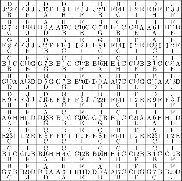
We compute a 10×10 pattern obtained by coding the orbit of some starting point under the ℤ2-action R0.
sage: from slabbe.coding_of_PETs import PETsCoding
sage: coding_R0_P = PETsCoding((R0e1,R0e2), P)
sage: pattern = coding_R0_P.pattern((.3,.4), (10,10))
sage: pattern = WangTiling(pattern, T0)
sage: pattern.tikz()
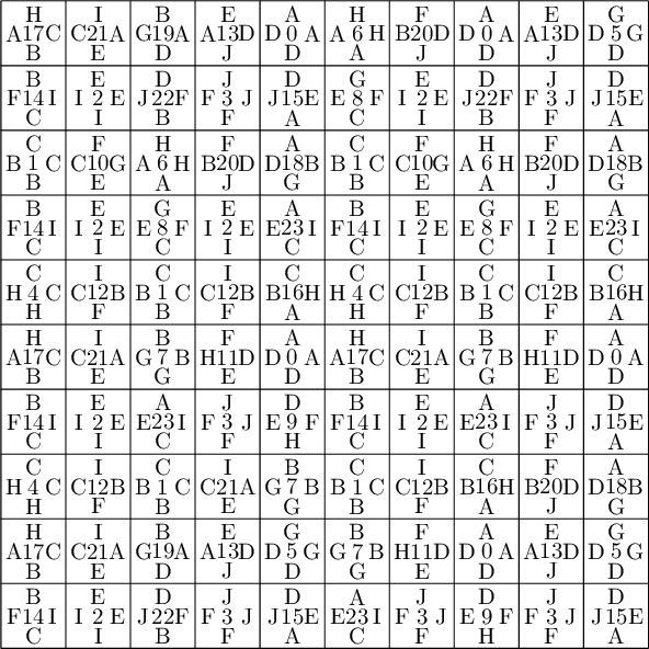
We observe that this pattern is not valid !!!
Let's fix the partition
We claim that the above pattern is wrong because something is wrong in the labelling of the atoms in the partition proposed by Jang and Robinson for the 24 Wang tiles encoding Penrose tilings.
Below, we fix the partition by swapping labels 8 and 23, 9 and 22, 11 and 20, 10 and 21:
sage: d = {i:i for i in range(24)}
sage: d.update({8:23, 23:8, 9:22, 22:9, 11:20, 20:11, 10:21, 21:10})
sage: P1 = P.rename_keys(d)
sage: P1.plot()
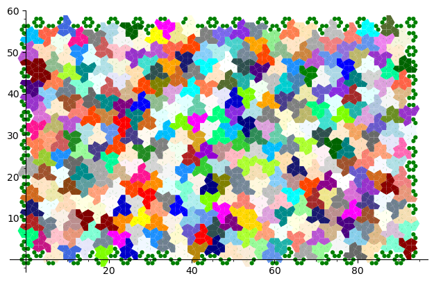
We compute a 10×10 pattern out of this updated partition P1:
sage: coding_R0_P1 = PETsCoding((R0e1,R0e2), P1)
sage: pattern = coding_R0_P1.pattern((.3,.4), (10,10))
sage: pattern = WangTiling(pattern, T0)
sage: pattern.tikz()
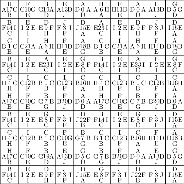
We observe that this pattern is valid !!!
Understanding the issue using edge label partitions
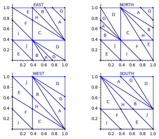
Let us try to understand the fix in terms of the Wang tiles east, north, west and south edge labels partitions induced by the original partition.
Indeed, since each atom of the partition corresponds to a Wang tile, we can deduce a partition of the unit square for the east labels (and respectively for the north, west and south labels) by merging two atoms in the partition if their east edge label is the same.
sage: def edge_label_partitions(partition, tiles):
....:     EAST = partition.merge_atoms({i:tiles[i][0] for i in range(24)})
....:     NORTH = partition.merge_atoms({i:tiles[i][1] for i in range(24)})
....:     WEST = partition.merge_atoms({i:tiles[i][2] for i in range(24)})
....:     SOUTH = partition.merge_atoms({i:tiles[i][3] for i in range(24)})
....:     return EAST, NORTH, WEST, SOUTH
sage: def draw_edge_label_partitions(partition, tiles):
....:     EAST, NORTH, WEST, SOUTH = edge_label_partitions(partition, tiles)
....:     L = [EAST.plot() + text('EAST', (.5,1.05)),
....:          NORTH.plot() + text('NORTH', (.5,1.05)),
....:          WEST.plot() + text('WEST', (.5,1.05)),
....:          SOUTH.plot() + text('SOUTH', (.5,1.05))]
....:     return graphics_array(L, nrows=2)
This is what we get using the partition proposed by Jang and Robinson for the 24 Wang tiles encoding Penrose tilings:
sage: draw_edge_label_partitions(P, T0)
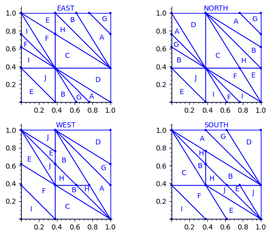
Here are some observations which are normal:
- partitions NORTH and EAST are symmetric under a reflexion by the positive diagonal (remember that the tile set is symmetric under the positive diagonal)
- partitions WEST and SOUTH are symmetric under a reflexion by the positive diagonal (remember that the tile set is symmetric under the positive diagonal)
Here are some observations which are not normal:
- partitions WEST and EAST do not give the same area to the same index (in a Wang tiling, the frequency of a EAST label should be equal to the frequency of the same WEST label)
- partitions SOUTH and NORTH do not give the same area to the same index (in a Wang tiling, the frequency of a NORTH label should be equal to the frequency of the same SOUTH label)
- partitions EAST and WEST are not a translate of one another (idealy a horizontal translate)
- partitions SOUTH and NORTH are not a translate of one another (idealy a vertical translate)
Another indication that something may be wrong is:
- atoms B, H, E, J, A, G are not convex in the torus
This is not a necessity. Atoms are not convex in the Markov partition associated to Jeandel-Rao tilings [2]. But they are convex for the Ammann set of 16 Wang tiles and their generalization to metallic mean numbers made in [3,4]. Since Penrose tilings are closely related to Ammann A2 tilings, we may also expect to have simple convex atoms in each of the four edge label partitions.
Here is the area of each atom in each of the four partitions. We observe that only atoms C and D have the same area in each of the four partitions.
sage: def table_of_area_of_atom_in_east_north_west_south_partitions(partition, tiles):
....:     columns = []
....:     labels = 'ABCDEFGHIJ'
....:     EAST, NORTH, WEST, SOUTH = edge_label_partitions(partition, tiles)
....:     for partition in [EAST, NORTH, WEST, SOUTH]:
....:         d = partition.volume_dict()
....:         column = [d[a] for a in labels]
....:         columns.append(column)
....:     header_row = ['EAST', 'NORTH', 'WEST', 'SOUTH']
....:     return table(columns=columns, header_row=header_row, header_column=['']+list(labels))
sage: table_of_area_of_atom_in_east_north_west_south_partitions(P, T0)
    │ EAST             NORTH            WEST             SOUTH
├───┼────────────────┼────────────────┼────────────────┼────────────────┤
  A │ 15/2*phi - 12    15/2*phi - 12    phi - 3/2        phi - 3/2
  B │ phi - 3/2        phi - 3/2        15/2*phi - 12    15/2*phi - 12
  C │ phi - 3/2        phi - 3/2        phi - 3/2        phi - 3/2
  D │ phi - 3/2        phi - 3/2        phi - 3/2        phi - 3/2
  E │ phi - 3/2        phi - 3/2        -11/2*phi + 9    -11/2*phi + 9
  F │ -11/2*phi + 9    -11/2*phi + 9    phi - 3/2        phi - 3/2
  G │ -8*phi + 13      -8*phi + 13      -3/2*phi + 5/2   -3/2*phi + 5/2
  H │ -3/2*phi + 5/2   -3/2*phi + 5/2   -8*phi + 13      -8*phi + 13
  I │ 5*phi - 8        5*phi - 8        -3/2*phi + 5/2   -3/2*phi + 5/2
  J │ -3/2*phi + 5/2   -3/2*phi + 5/2   5*phi - 8        5*phi - 8
But, we observe that we can fix the partitions if we assume that the atoms C and D in the four partitions are correct. There is a unique translation sending atoms C,D in the partition WEST to the atoms C and D in the partition EAST. That translation should send the partition WEST exactly on EAST. Similarly for SOUTH and NORTH. This suggest a way to fix atoms B, H, E, J, A, G in the partition.
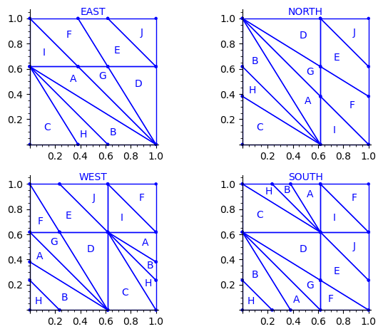
Fixed Edge labels partitions
Using the fixed partition, here is what we get.
sage: P1.plot()

sage: draw_edge_label_partitions(P1, T0)
Now it looks good! As for the partitions associated to the metallic mean Wang tiles, the four partitions are isometric copies of the other ones (under toral translation or reflection).
sage: table_of_area_of_atom_in_east_north_west_south_partitions(P1, T0)
    │ EAST             NORTH            WEST             SOUTH
├───┼────────────────┼────────────────┼────────────────┼────────────────┤
  A │ phi - 3/2        phi - 3/2        phi - 3/2        phi - 3/2
  B │ phi - 3/2        phi - 3/2        phi - 3/2        phi - 3/2
  C │ phi - 3/2        phi - 3/2        phi - 3/2        phi - 3/2
  D │ phi - 3/2        phi - 3/2        phi - 3/2        phi - 3/2
  E │ phi - 3/2        phi - 3/2        phi - 3/2        phi - 3/2
  F │ phi - 3/2        phi - 3/2        phi - 3/2        phi - 3/2
  G │ -3/2*phi + 5/2   -3/2*phi + 5/2   -3/2*phi + 5/2   -3/2*phi + 5/2
  H │ -3/2*phi + 5/2   -3/2*phi + 5/2   -3/2*phi + 5/2   -3/2*phi + 5/2
  I │ -3/2*phi + 5/2   -3/2*phi + 5/2   -3/2*phi + 5/2   -3/2*phi + 5/2
  J │ -3/2*phi + 5/2   -3/2*phi + 5/2   -3/2*phi + 5/2   -3/2*phi + 5/2
sage: (phi-3/2).n(), (-3/2*phi + 5/2).n()
(0.118033988749895, 0.0729490168751576)
Labels A, B, C, D, E and F all have the same frequency of ϕ − (3)/(2) ≈ 0.118.
Labels G, H, I and J all have the same frequency of − (3)/(2)ϕ + (5)/(2) ≈ 0.0729.
We check that frequencies sum to 1:
sage: 6 * (phi-3/2) + 4 * (-3/2*phi + 5/2)
1
Proposed partition for the encoding of the Penrose tilings into 24 Wang tiles
As done with the Markov partition associated to Jeandel-Rao aperiodic tilings, and for the Markov partition associated to the family of metallic mean Wang tiles, I think it is more natural to associate horizontal (vertical) translations in the internal space with horizontal (vertical) translations in the physical space. This way, the brain is less mixed up and the projections in the physical space π and in the internal space πint of the cut and project scheme are defined more naturally. This way the internal space and physical space can even be identified: this is the root of the do-it-yourself tutorial allowing the construction of Jeandel-Rao tilings [5]. See also my Habilitation à diriger des recherches written in English during Spring 2025 for more information [6].
First, we flip the partition P1 by the positive diagonal. This exchanges the role of x and y axis.
sage: P2 = P1.apply_linear_map(matrix(2, [0,1,1,0]))
sage: P2.plot()

This allows to define the ℤ2-action R1 on the torus with horizontal and vertical translations for e1 and e2 respectively:
sage: base = diagonal_matrix((1,1))
sage: R1e1 = PET.toral_translation(base, vector((1/phi,0)))
sage: R1e2 = PET.toral_translation(base, vector((0,1/phi)))
Then, we rotate the partition. This changes the origin of the partition. This change may be optional, but it makes the partition look closer to the partitions already studied in [2,3,4]. It simplifies the explanation of any relation between them (and there is one, see below!).
sage: P3 = R1e1(P2)
sage: P3 = R1e2(P3)
sage: P3.plot()
We observe that the partition P3 associated to the 24 Wang tiles encoding Penrose tiling is a refinement of the partition associated to the 16 Ammann tiles (see Figure 15 in [4] as the 16 Ammann tiles are equivalent to the n-th metallic mean Wang tiles when n = 1).
We compute a 10×10 pattern obtained by coding the orbit of some starting point under the ℤ2-action R1 using partition P3.
sage: from slabbe.coding_of_PETs import PETsCoding
sage: coding_R1_P3 = PETsCoding((R1e1,R1e2), P3)
sage: pattern = coding_R1_P3.pattern((.3,.4), (10,10))
sage: pattern = WangTiling(pattern, T0)
sage: pattern.tikz()
We are happy to see that the pattern is still valid after all the changes we have made!
sage: draw_edge_label_partitions(P3, T0)
We observe that the EAST, NORTH, WEST and SOUTH partitions are a refinement of the EAST, NORTH, WEST and SOUTH partitions associated to the Ammann tiles partition (see Figure 15 in [4]).
The difference between the Ammann EAST and 24 Wang tiles Penrose EAST partition is the addition of two closed geodesics of slope -1 on the 2-torus passing through the origin and through the vertex (0, φ − 1).
It is possible that there is a clever way of including this information into the labels of the Wang tiles as we have done it for the family of metallic mean Wang tiles. Possibly, we need to use 4-dimension vectors for the tile labels instead of 3-dimensional integer vectors. This remains an open question.
Wang tiles deduced from the partition and ℤ2-action
We check that the Wang tiles computed from the partition P3 and ℤ2-action R1 is the original set of 24 Wang tiles defined by Jang and Robinson.
See Proposition 8.1 in [2].
sage: T = coding_R1_P3.to_wang_tiles()
sage: T.tikz()
sage: T.is_equivalent(T0, certificate=True)
(True,
 {'3': 'D',
  '0': 'A',
  '6': 'G',
  '1': 'B',
  '7': 'H',
  '2': 'C',
  '8': 'I',
  '4': 'E',
  '5': 'F',
  '9': 'J'},
 {'3': 'D',
  '0': 'A',
  '6': 'G',
  '1': 'B',
  '7': 'H',
  '2': 'C',
  '8': 'I',
  '4': 'E',
  '5': 'F',
  '9': 'J'},
 Substitution 2d: {0: [[0]], 1: [[1]], 2: [[2]], 3: [[3]], 4: [[4]], 5:
 [[5]], 6: [[6]], 7: [[7]], 8: [[8]], 9: [[9]], 10: [[10]], 11: [[11]], 12:
 [[12]], 13: [[13]], 14: [[14]], 15: [[15]], 16: [[16]], 17: [[17]], 18: [[18]],
 19: [[19]], 20: [[20]], 21: [[21]], 22: [[22]], 23: [[23]]})
Introduction to Python/SageMath
27 juin 2023 | Catégories: sage, math | View CommentsOn Wednesday June 28th, 2023, I give short a Introduction to Python/SageMath as an online course organized by Pierre-Guy Plamondon in Mathematical Summer in Paris (MSP23) on WorkAdventure. Below is the material that will be presented or suggested.
Exercises:
- Install and open a Jupyter notebook and do the User Interface Tour in the help menu.
- Programming with Python. Here is a list of Jupyter notebooks to learn programming in Python: ProgrammingExercises.zip or ProgrammingExercises.tar.xz
- Reproduce the computations made by BuzzFeedNews in a github repository of your choice, for instance about the fentanyl and cocaine overdose deaths (2018) or about The Tennis Racket (2016).
- Solve some problems from the Project Euler. Project Euler contains more than 500 exercises that have to be solved with a computer
- Reproduce one or more images from the matplotlib library.
- Download the book Mathematical Computation with Sage by Paul Zimmermann et al. about the SageMath open source software. Reproduce the computations made in a section of your choice in the book.
- Visit https://ask.sagemath.org/questions/ and try to reproduce some of the best answers to questions of interest for you.
- Choose a section of your choice in the SageMath very large Reference Manual and reproduce the computations made in it.
When working on the above, two principles applies:
- Once you finished solving a notebook or a problem on Project Euler on your own you need to explain your solution to at least one other person (who has already solved the same notebook or problem).
- Once you reproduced the computation made by BuzzFeedNews, matplotlib image or some computation, you need to present and explain it to at least one other person.
Supplementary material:
- Experimenting with Dynamical systems in SageMath: DynamicalSystemExercices.zip
- Some more notebooks and exercices from this course given by Vincent Delecroix at AIMS in Rwanda (2016).
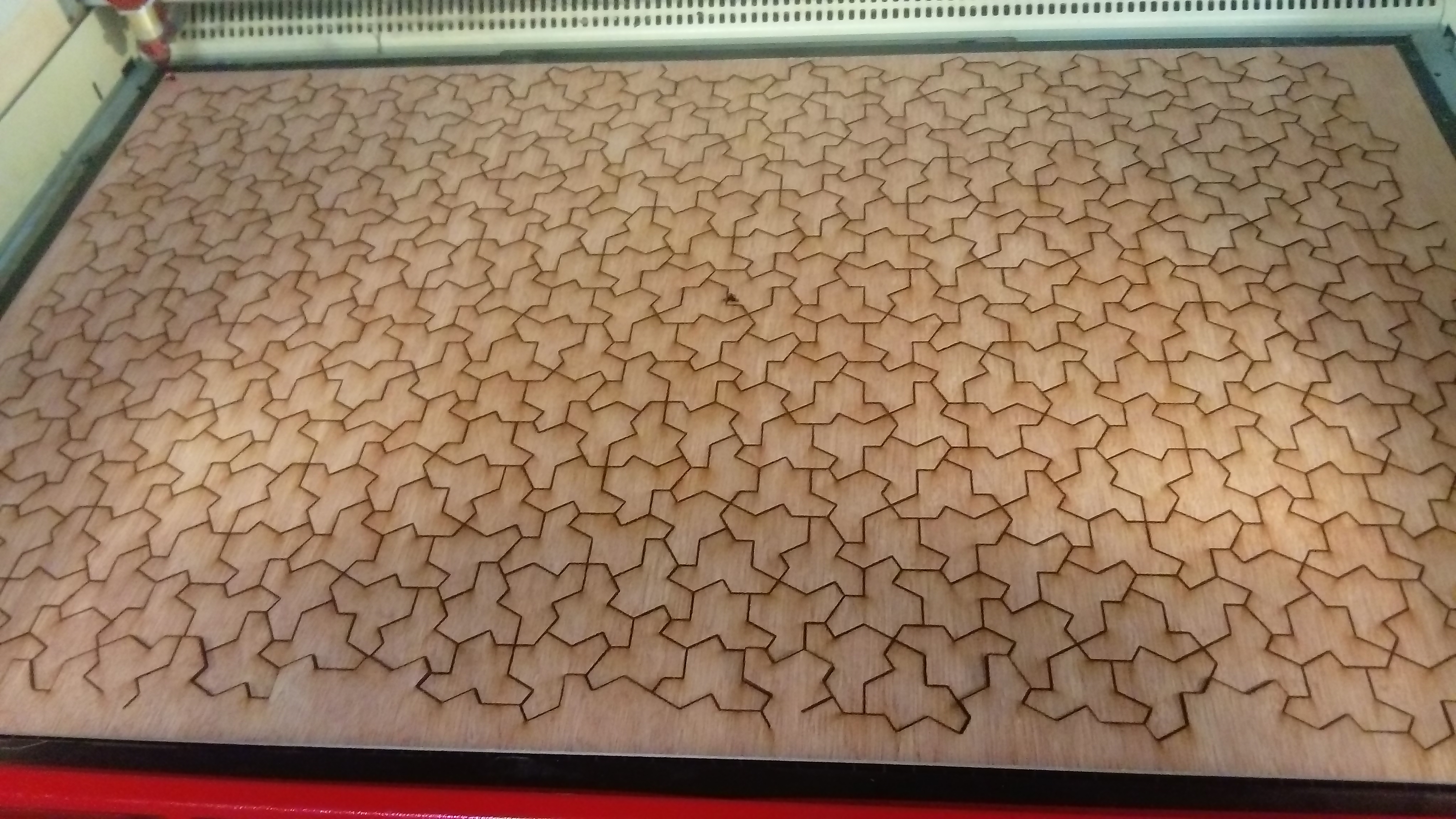
Découpe laser du chapeau, tuile apériodique découverte récemment
25 mai 2023 | Catégories: sage, slabbe spkg, math, découpe laser | View CommentsLe chapeau est une tuile apériodique découverte par David Smith, Joseph Samuel Myers, Craig S. Kaplan, et Chaim Goodman-Strauss le 20 mars 2023. Suite à un exposé donné le 26 mars au National Museum of Mathematics, la nouvelle s'est vite répandue. En effet, cette découverte a été mentionnée les jours suivants dans des blogues puis dans Le New York Times le 28 mars, Le Monde le 29 mars, puis The Guardian et QuantaMagazine le 4 avril. Un vidéo de 20 minutes, réalisé par Passe-Science et publié début le 3 mai, explique le résultat et son contexte.
Déjà des articles proposant des résultats plus approfondis sur la tuile par des experts du domaine sont parus sur arXiv en mai 2023. Ils interprêtent les pavages comme des coupes et projection de réseaux de dimension supérieure. Le deuxième propose même une partition de la fenêtre de l'espace interne, un peu comme pour les pavages de Jeandel-Rao, à la différence qu'ici la partition a des bords fractales ce qui est pour moi une grande surprise.
Comme je faisais une intervention dans l'école de mon garçon à Bègles le 3 mai et au Lycée Kastler de Talence le 4 mai, j'ai réalisé un projet de découpe laser sur la tuile apériodique afin de partager cette récente découverte.
La première question était de construire un pavage d'un rectangle assez grand avec la pièce apériodique. Pour ce faire, j'ai ajouté un nouveau module dans mon package optionel au logiciel SageMath.
Le module réalise une réduction à une instance du problème de la couverture universelle, qui peut être résolu dans SageMath en utilisant l'algorithme des liens dansants de Donald Knuth, les solveurs SAT ou les programmes d'optimisation linéaire (solveur MILP). Le code utilise le système de coordonnées défini dans le fichier validate/kitegrid.pdf qui se trouve dans le code source associé à l'article.
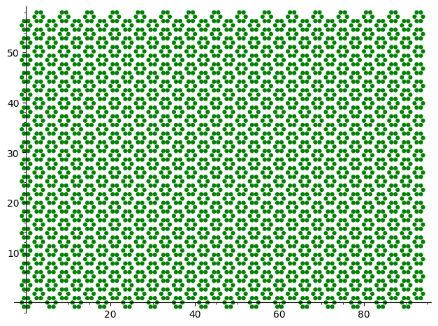
Voici un exemple de construction d'un pavage avec la tuile apériodique. Le calcul est fait dans le logiciel SageMath muni de la version de développement de mon package optionnel slabbe qui peut être installé avec la commande sage -pip install slabbe. Ici, j'utilise le solveur SAT Glucose, développé au LaBRI. On peut installer glucose dans SageMath avec la commande sage -i glucose.
sage: from slabbe.aperiodic_monotile import MonotileSolver
sage: s = MonotileSolver(16, 17)
sage: G = s.draw_one_solution(solver='glucose')
sage: G.save('solution_16x17.png')
sage: G
Dans la manière de résoudre la question ci-haut, le problème est représenté par un problème de couverture exacte qui consiste à recouvrir exactement les entiers de 1 à n avec des sous-ensembles choisis dans une liste de sous-ensembles déterminés. Ici, on représente l'espace à recouvrir de manière discrète en comptant 6 points du plan par hexagone (un point pour chaque kite contenu dans un hexagone). Rappelons que la pièce Chapeau qui nous intéresse est formée d'une union d'exactement 8 de ces kites.
sage: s.plot_domain()
Ensuite, on construit une matrice de 0 et de 1 avec autant de colonnes que de points ci-haut (16 * 17 * 2 * 6 = 3264) et autant de lignes qu'il y a de copies isométriques de la pièce intersectant le domaine. Pour chaque copie de la pièce, une ligne dans la matrice contient des 1 exactement dans les colonnes associées aux kites occupés par la pièce.
sage: s.the_dlx_solver()
Dancing links solver for 3264 columns and 7116 rows
Le calcul ci-haut qui a construit la matrice (sparse) indique qu'il y a 7116 copies isométriques de la pièce qui intersectent (complètement ou partiellement) le domaine. Quand on voudra dessiner une solution, on ignorera les pièces incomplètes.
On peut maintenant résoudre le problème.
sage: s = MonotileSolver(8,8)
sage: %time L = s.one_solution()   # l'algo des liens dansants de Knuth est utilisé par défaut
CPU times: user 798 ms, sys: 32.2 ms, total: 830 ms
Wall time: 1min 20s
Le contenu d'une solution est une liste de nombres indiquant les lignes de la matrice de 0/1 à considérer pour former une solution. C'est-à-dire que la sous-matrice restreinte aux lignes données comporte exactement un 1 dans chaque colonne:
sage: L
[81,
 85,
 125,
 128,
 ...
 1772,
 1783,
 1794,
 1815]
Ici, il se trouve que les solveurs SAT sont plus efficaces que l'algo des liens dansants pour trouver une solution:
sage: %time L = s.one_solution(solver='glucose')
CPU times: user 326 ms, sys: 16.1 ms, total: 342 ms
Wall time: 526 ms
sage: %time L = s.one_solution(solver='kissat')
CPU times: user 335 ms, sys: 3.64 ms, total: 339 ms
Wall time: 461 ms
En effet, Glucose se comporte plutôt bien pour résoudre des problèmes de pavages du plan lorsqu'il existe une solution. Mais lorsqu'il n'y a pas de solution, l'algo des liens dansants de Knuth est parfois mieux. Aussi, l'algo des liens dansants de Knuth est très efficace pour énumérer toutes les solutions.
Le solveur Kissat a été ajouté dans SageMath par moi-même comme package optionnel cette année suite à une discussion avec Laurent Simon au café du LaBRI. On peut installer le solveur kissat dans SageMath avec la commande sage -i kissat.
Ici on extrait le contour des pièces d'une solution (tel que chaque arête est dessinée une seule fois afin d'éviter que la découpeuse laser passe deux fois par chaque arête ce qui peut endommager ou brûler le bord des pièces en bois) et on crée un fichier pdf ou svg. Je choisis une taille de 16 double-hexagones horizontalement et 17 verticalement, car cela crée un fichier qui correspond à une taille de 1m x 60cm. C'est la taille de la découpeuse laser à notre disposition:
sage: s = MonotileSolver(16, 17)
sage: tikz = s.one_solution_tikz(solver='glucose')
sage: tikz.pdf('solution_16x17.pdf')
sage: tikz.svg('solution_16x17.svg')     # or
Avec l'aide de David Renault, mon collègue du LaBRI qui enseigne à l'ENSEIRB et qui m'a déjà accompagné dans la réalisation de projets de découpe laser, nous avons découpé le fichier ci-haut le jeudi 27 avril au EirLab, l'atelier de fabrication numérique (FabLab) de l'ENSEIRB-MATMECA:
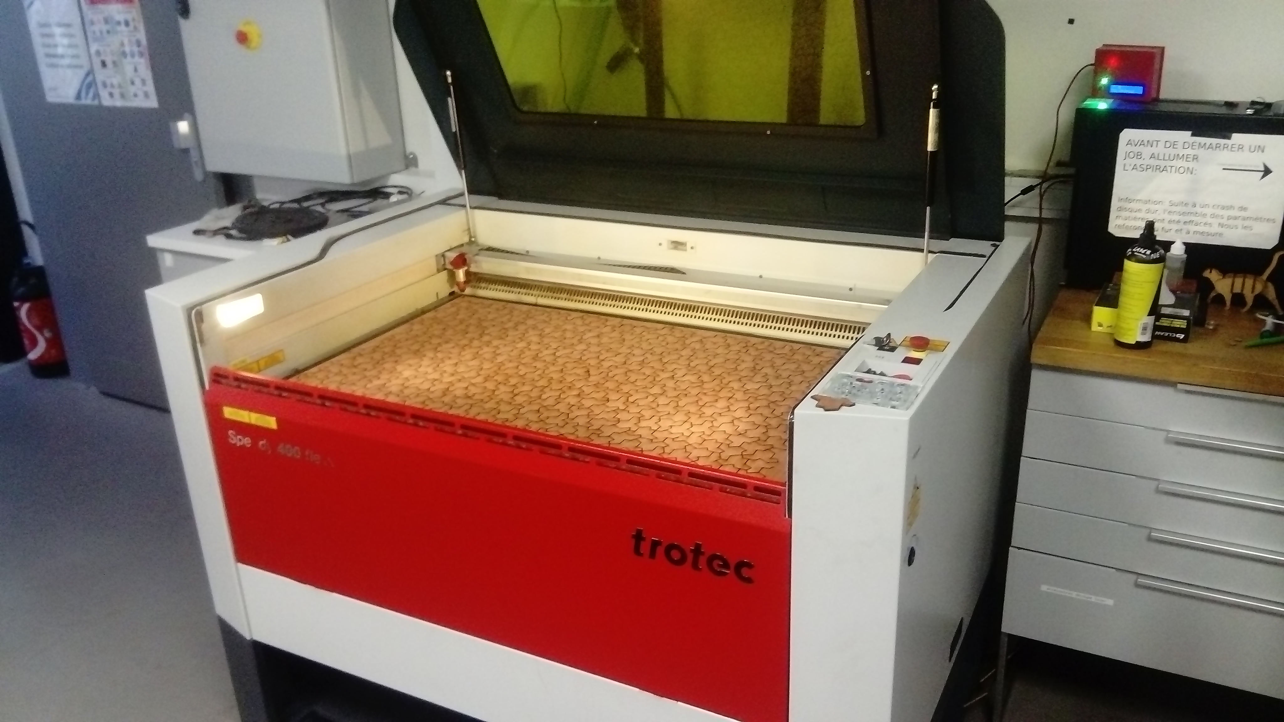
Comme toujours, il faut quelque peu modifier le fichier svg dans Inkscape avant de lancer la découpe laser. Voici le fichier modifié juste avant la découpe.
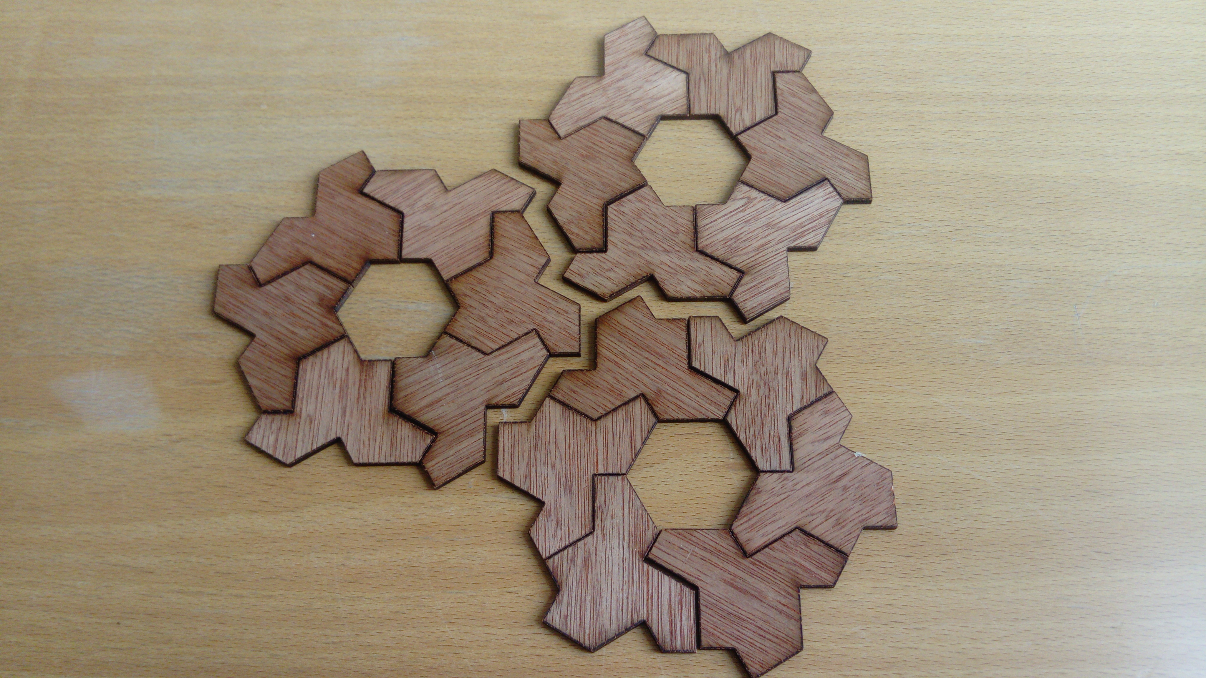
Maintenant, on peut s'amuser avec les pièces:
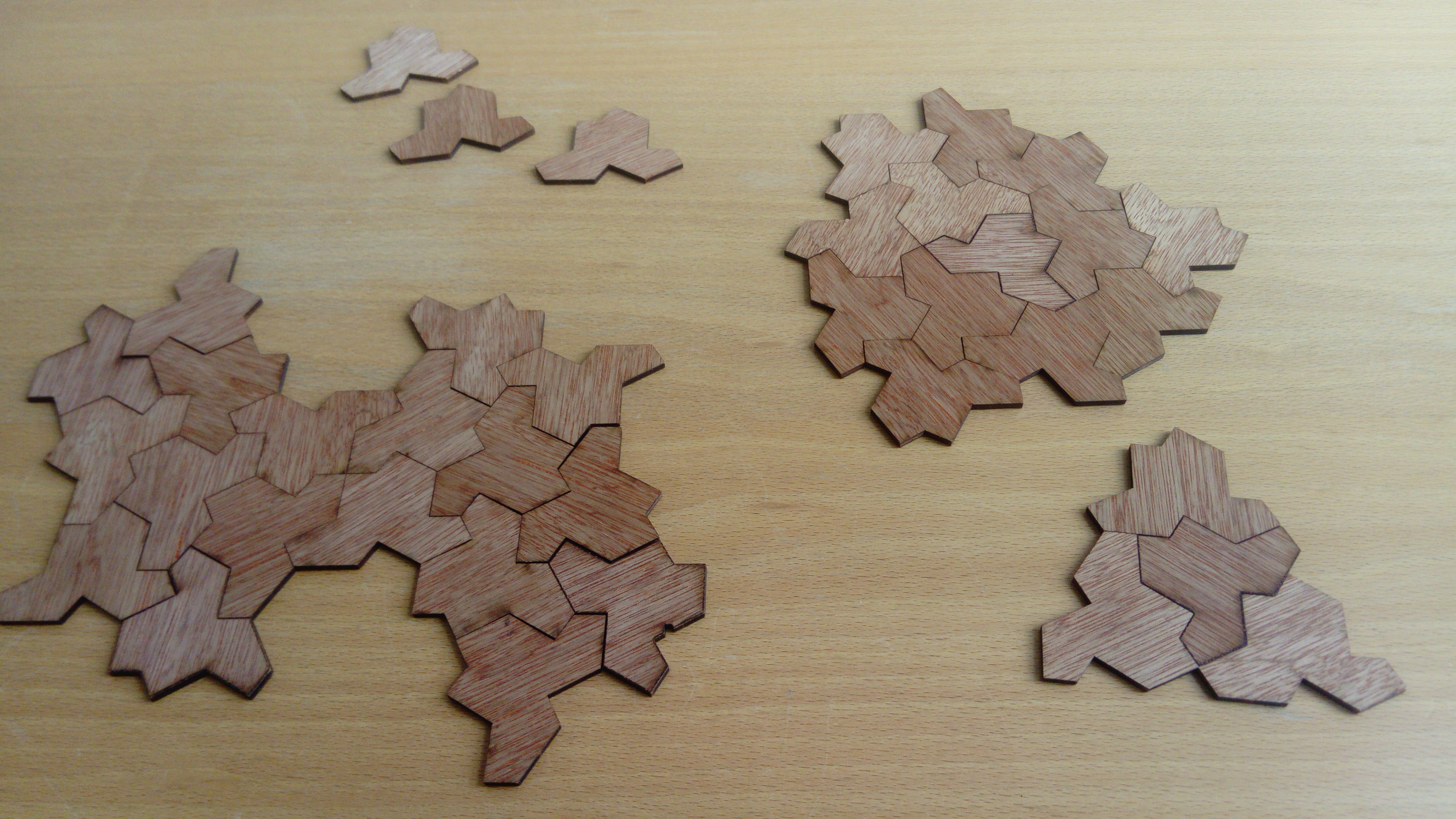
Avec mes garçons, nous avons trouvé une forme intéressante qui recouvre le plan périodiquement à l'exception d'un trou hexagonal. Il se trouve que la même forme peut-être créée de deux façons différentes: sur l'image ci-bas la forme à droite est la globalement la même, mais elle n'est pas obtenue de la même façon que celle en haut à gauche. Pourtant, toutes deux ont le même contour extérieur et le même trou hexagonal.
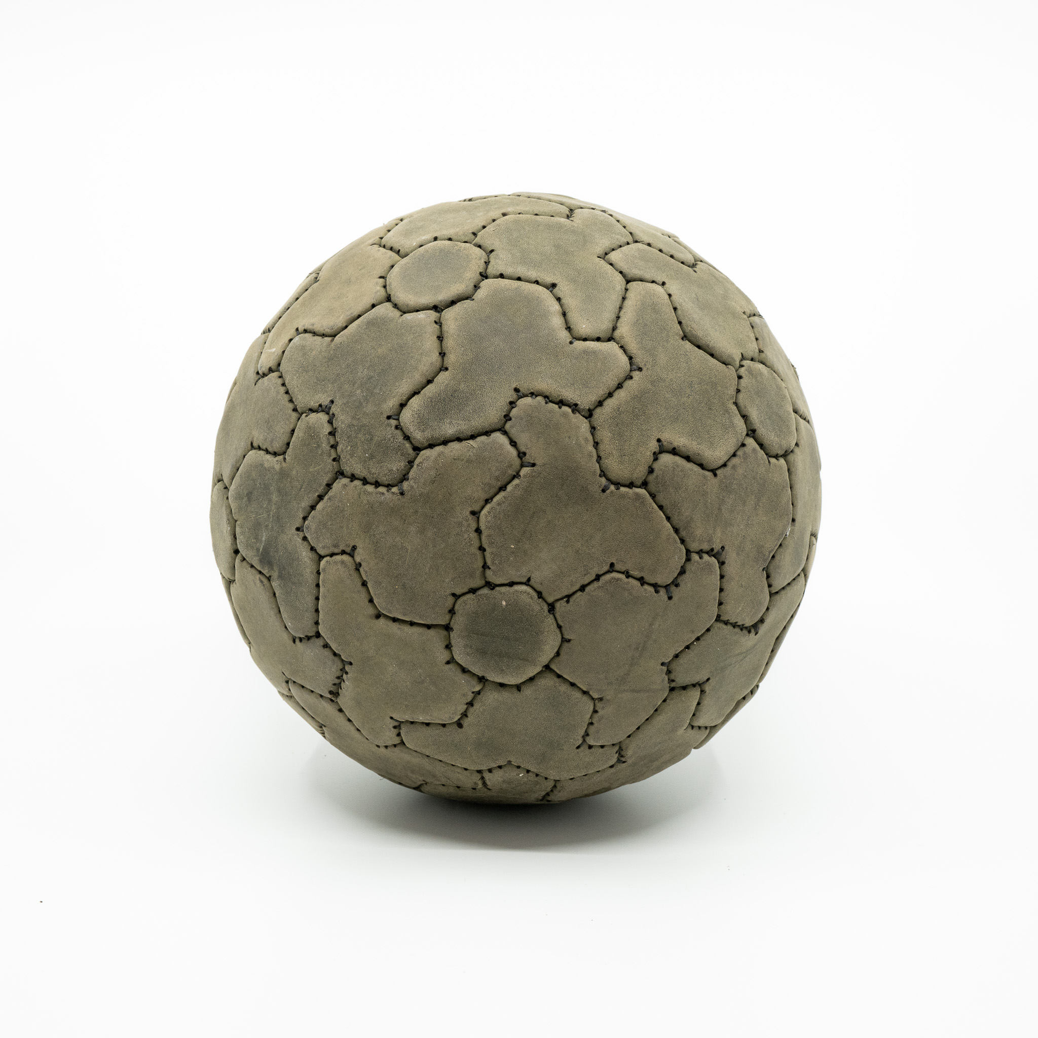
Cette observation, déjà faite par d'autres, a mené au recouvrement d'une sphère avec la pièce et un trou pentagonal:
Factor complexity of words generated by multidimensional continued fraction algorithms
03 novembre 2022 | Catégories: sage | View CommentsI was asked by email how to compute with SageMath the factor complexity of words generated by multidimensional continued fraction algorithms. I'm copying my answer here so that I can more easily share it.
A) How to calculate the factor complexity of a word
To compute the complexity in factors, we need a finite word and not an infinite infinite word. In the example below, I take a prefix of the Fibonacci word and I compute the number of factors of size 100 and of size 0 to 19:
sage: w = words.FibonacciWord()
sage: w
word: 0100101001001010010100100101001001010010...
sage: prefix = w[:100000]
sage: prefix.number_of_factors(100)
101
sage: [prefix.number_of_factors(i) for i in range(20)]
[1, 2, 3, 4, 5, 6, 7, 8, 9, 10, 11, 12, 13, 14, 15, 16, 17, 18, 19, 20]
The documentation for the number_of_factors method contains more examples, etc.
B) How to construct an S-adic word in SageMath
The method words.s_adic in SageMath allows to construct an S-adic sequence from a directive sequence, a set of substitutions and a sequence of first letters.
For example, we may use Kolakoski word as a directive sequence:
sage: directive_sequence = words.KolakoskiWord()
sage: directive_sequence
word: 1221121221221121122121121221121121221221...
Then, I define the Thue-Morse and Fibonacci substitutions:
sage: tm = WordMorphism('a->ab,b->ba')
sage: fib = WordMorphism('a->ab,b->a')
sage: tm
WordMorphism: a->ab, b->ba
sage: fib
WordMorphism: a->ab, b->a
Then, to define an S-adic sequence, I also need to define the sequence of first letters. Here, it is always the constant sequence a,a,a,a,...:
sage: from itertools import repeat
sage: letters = repeat('a')
I associate the letter 1 in the Kolakoski sequence to the Thue-Morse morphism and 2 to the Fibonacci morphism, this allows to construct an S-adic sequence:
sage: w = words.s_adic(directive_sequence, letters, {1:tm, 2:fib})
sage: w
word: abbaababbaabbaabbaababbaabbaababbaababba...
Then, as above, I can take a prefix and compute its factor complexity:
sage: prefix = w[:100000]
sage: [prefix.number_of_factors(i) for i in range(20)]
[1, 2, 4, 6, 7, 8, 9, 10, 12, 14, 16, 18, 20, 22, 24, 26, 28, 30, 34, 38]
C) Creating an S-adic sequence from Brun algorithm
With the package slabbe, you can construct an S-adic sequence from some of the known Multidimensional Continued Fraction Algorithm.
One can install it by running sage -pip install slabbe in a terminal where sage command exists. Sometimes this does not work.
Then, one may do:
sage: from slabbe.mult_cont_frac import Brun
sage: algo = Brun()
sage: algo
Brun 3-dimensional continued fraction algorithm
sage: D = algo.substitutions()
sage: D
{312: WordMorphism: 1->12, 2->2, 3->3,
 321: WordMorphism: 1->1, 2->21, 3->3,
 213: WordMorphism: 1->13, 2->2, 3->3,
 231: WordMorphism: 1->1, 2->2, 3->31,
 123: WordMorphism: 1->1, 2->23, 3->3,
 132: WordMorphism: 1->1, 2->2, 3->32}
sage: directive_sequence = algo.coding_iterator((1,e,pi))
sage: [next(directive_sequence) for _ in range(10)]
[123, 312, 312, 321, 132, 123, 312, 231, 231, 213]
Construction of the s-adic word from the substitutions and the directive sequence:
sage: from itertools import repeat
sage: D = algo.substitutions()
sage: directive_sequence = algo.coding_iterator((1,e,pi))
sage: words.s_adic(directive_sequence, repeat(1), D)
word: 1232323123233231232332312323123232312323...
Shortcut:
sage: algo.s_adic_word((1,e,pi))
word: 1232323123233231232332312323123232312323...
There are some more examples in the documentation.
This code was used in the creation of the 3-dimensional Continued Fraction Algorithms Cheat Sheets 7 years ago during my postdoc at Université de Liège, Belgium.
Using Glucose SAT solver to find a tiling of a rectangle by polyominoes
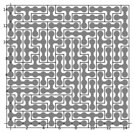
27 mai 2021 | Mise à jour: 20 juin 2022 | Catégories: sage, math | View CommentsIn his Dancing links article, Donald Knuth considered the problem of packing 45 Y pentaminoes into a 15 x 15 square. We can redo this computation in SageMath using some implementation of his dancing links algorithm.
Dancing links takes 1.24 seconds to find a solution:
sage: from sage.combinat.tiling import Polyomino, TilingSolver
sage: y = Polyomino([(0,0),(1,0),(2,0),(3,0),(2,1)])
sage: T = TilingSolver([y], box=(15, 15), reusable=True, reflection=True)
sage: %time solution = next(T.solve())
CPU times: user 1.23 s, sys: 11.9 ms, total: 1.24 s
Wall time: 1.24 s
The first solution found is:
sage: sum(T.row_to_polyomino(row_number).show2d() for row_number in solution)
What is nice about dancing links algorithm is that it can list all solutions to a problem. For example, it takes less than 3 minutes to find all solutions of tiling a 15 x 15 rectangle with the Y polyomino:
sage: %time T.number_of_solutions()
CPU times: user 2min 46s, sys: 3.46 ms, total: 2min 46s
Wall time: 2min 46s
1696
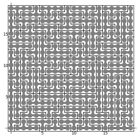
It takes more time (38s) to find a first solution of a larger 20 x 20 rectangle:
sage: T = TilingSolver([y], box=(20,20), reusable=True, reflection=True)
sage: %time solution = next(T.solve())
CPU times: user 38.2 s, sys: 7.88 ms, total: 38.2 s
Wall time: 38.2 s
The polyomino tiling problem is reduced to an instance of the universal cover problem which is represented by a sparse matrix of 0 and 1:
sage: dlx = T.dlx_solver()
sage: dlx
Dancing links solver for 400 columns and 2584 rows
We observe that finding a solution to this problem takes the same amount of time. This is normal since it is exactly what is used behind the scene when calling next(T.solve()) above:
sage: %time sol = dlx.one_solution(ncpus=1)
CPU times: user 38.6 s, sys: 48 ms, total: 38.6 s
Wall time: 38.5 s
One way to improve the time it takes it to split the problem into parts and use many processors to work on each subproblems. Here a random column is used to split the problem which may affect the time it takes. Sometimes a good column is chosen and it works great as below, but sometimes it does not:
sage: %time sol = dlx.one_solution(ncpus=2)
CPU times: user 941 µs, sys: 32 ms, total: 32.9 ms
Wall time: 1.41 s
The reduction from dancing links instance to SAT instance #29338 and to MILP instance #29955 was merged into SageMath 9.2 during the last year. A discussion with Franco Saliola motivated me to implement these translations since he was also searching for faster way to solve dancing links problems. Indeed some problems are solved faster with other kind of solver, so it is good to make some comparisons between solvers.
Therefore, with a recent enough version of SageMath, we can now try to find a tiling with other kinds of solvers. Following my experience with tilings by Wang tiles, I know that Glucose SAT solver is quite efficient to solve tilings of the plane. This is why I test this one below. Glucose is now an optional package to SageMath which can be installed with:
sage -i glucose
Update (June 20th, 2022): It seems sage -i glucose no longer works. The new procedure is to use ./configure --enable-glucose when installation is made from source. See the question Unable to install glucose SAT solver with Sage on ask.sagemath.org for more information.
Glucose finds the solution of a 20 x 20 rectangle in 1.5 seconds:
sage: %time sol = dlx.one_solution_using_sat_solver('glucose')
CPU times: user 306 ms, sys: 12.1 ms, total: 319 ms
Wall time: 1.51 s
The rows of the solution found by Glucose are:
sage: sol
[0, 15, 19, 38, 74, 245, 270, 310, 320, 327, 332, 366, 419, 557, 582, 613, 660,
 665, 686, 699, 707, 760, 772, 774, 781, 802, 814, 816, 847, 855, 876, 905,
 1025, 1070, 1081, 1092, 1148, 1165, 1249, 1273, 1283, 1299, 1354, 1516, 1549,
 1599, 1609, 1627, 1633, 1650, 1717, 1728, 1739, 1773, 1795, 1891, 1908, 1918,
 1995, 2004, 2016, 2029, 2037, 2090, 2102, 2104, 2111, 2132, 2144, 2146, 2185,
 2235, 2301, 2460, 2472, 2498, 2538, 2548, 2573, 2583]
Each row correspond to a Y polyomino embedded in the plane in a certain position:
sage: sum(T.row_to_polyomino(row_number).show2d() for row_number in sol)
Glucose-Syrup (a parallelized version of Glucose) takes about the same time (1 second) to find a tiling of a 20 x 20 rectangle:
sage: T = TilingSolver([y], box=(20, 20), reusable=True, reflection=True)
sage: dlx = T.dlx_solver()
sage: dlx
Dancing links solver for 400 columns and 2584 rows
sage: %time sol = dlx.one_solution_using_sat_solver('glucose-syrup')
CPU times: user 285 ms, sys: 20 ms, total: 305 ms
Wall time: 1.09 s
Searching for a tiling of a 30 x 30 rectangle, Glucose takes 40s and Glucose-Syrup takes 16s while dancing links algorithm takes much longer (next(T.solve()) which is using dancing links algorithm does not halt in less than 5 minutes):
sage: T = TilingSolver([y], box=(30,30), reusable=True, reflection=True)
sage: dlx = T.dlx_solver()
sage: dlx
Dancing links solver for 900 columns and 6264 rows
sage: %time sol = dlx.one_solution_using_sat_solver('glucose')
CPU times: user 708 ms, sys: 36 ms, total: 744 ms
Wall time: 40.5 s
sage: %time sol = dlx.one_solution_using_sat_solver('glucose-syrup')
CPU times: user 754 ms, sys: 39.1 ms, total: 793 ms
Wall time: 16.1 s
Searching for a tiling of a 35 x 35 rectangle, Glucose takes 2min 5s and Glucose-Syrup takes 1min 16s:
sage: T = TilingSolver([y], box=(35, 35), reusable=True, reflection=True)
sage: dlx = T.dlx_solver()
sage: dlx
Dancing links solver for 1225 columns and 8704 rows
sage: %time sol = dlx.one_solution_using_sat_solver('glucose')
CPU times: user 1.07 s, sys: 47.9 ms, total: 1.12 s
Wall time: 2min 5s
sage: %time sol = dlx.one_solution_using_sat_solver('glucose-syrup')
CPU times: user 1.06 s, sys: 24 ms, total: 1.09 s
Wall time: 1min 16s
Here are the info of the computer used for the above timings (a 4 years old laptop runing Ubuntu 20.04):
$ lscpu
Architecture :                          x86_64
Mode(s) opératoire(s) des processeurs : 32-bit, 64-bit
Boutisme :                              Little Endian
Address size :                          39 bits physical, 48 bits virtual
Processeur(s) :                         8
Liste de processeur(s) en ligne :       0-7
Thread(s) par coeur :                   2
Coeur(s) par socket :                   4
Socket(s) :                             1
Noeud(s) NUMA :                         1
Identifiant constructeur :              GenuineIntel
Famille de processeur :                 6
Modèle :                                158
Nom de modèle :                         Intel(R) Core(TM) i7-7820HQ CPU @ 2.90GHz
Révision :                              9
Vitesse du processeur en MHz :          3549.025
Vitesse maximale du processeur en MHz : 3900,0000
Vitesse minimale du processeur en MHz : 800,0000
BogoMIPS :                              5799.77
Virtualisation :                        VT-x
Cache L1d :                             128 KiB
Cache L1i :                             128 KiB
Cache L2 :                              1 MiB
Cache L3 :                              8 MiB
Noeud NUMA 0 de processeur(s) :         0-7
To finish, I should mention that the implementation of dancing links made in SageMath is not the best one. Indeed, according to what Franco Saliola told me, the dancing links code written by Donald Knuth himself and available on his website (franco added some makefile to compile it more easily) is faster. It would be interesting to confirm this and if possible improves the implementation made in SageMath.
Next Page »
Propulsé par Blogofile
S'abonner au Flux RSS
et aux Commentaires.

This work by Sébastien Labbé is licensed under a Creative Commons Attribution-ShareAlike 4.0 International License.