Dependencies

The computations made here depend on the modules WangTileSet, WangTiling, PolyhedronPartition, PolyhedronExchangeTransformation, PETsCoding implemented in the SageMath optional package slabbe over the last years in order to describe and study the Jeandel-Rao aperiodic tilings and the family of metallic mean Wang tiles.

Note that the package slabbe can be installed by running !pip install slabbe directly in SageMath:

sage: # !pip install slabbe             # uncomment and execute this line to install slabbe package

Here are the version of the packages used in this post:

sage: import importlib
sage: importlib.metadata.version("slabbe")
'0.8.0'

sage: version()
'SageMath version 10.5.beta6, Release Date: 2024-09-29'

Jang-Robinson encoding of the Penrose 24 Wang tiles

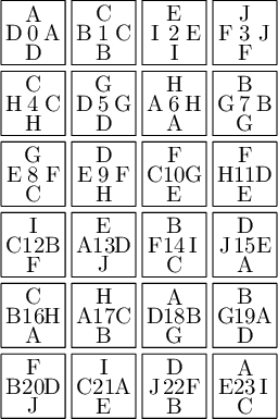
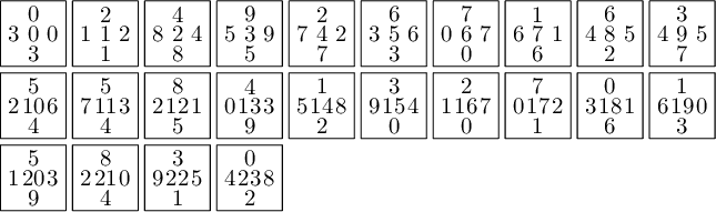
We encode the 24 Wang tiles proposed by Jang and Robinson (Figure 9 of [1]) using alphabet {A, B, C, D, E, F, G, H, I, J} for the shapes:

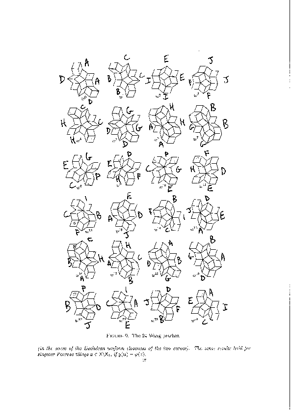
We define the 24 Wang tiles in SageMath:

sage: from slabbe import WangTileSet, WangTiling
sage: tiles = ["AADD", "CCBB", "EEII", "JJFF",
....:          "CCHH", "GGDD", "HHAA", "BBGG",
....:          "FGEC", "FDEH", "GFCE", "DFHE",
....:          "BICF", "DEAJ", "IBFC", "EDJA",
....:          "HCBA", "CHAB", "BADG", "ABGD",
....:          "DFBJ", "AICE", "FDJB", "IAEC"]
sage: T0 = WangTileSet([tuple(str(a) for a in tile) for tile in tiles])
sage: T0
Wang tile set of cardinality 24

sage: T0.tikz(ncolumns=4)

Constructing Jang-Robinson Bifurcation diagram as a polygonal partition

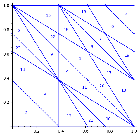
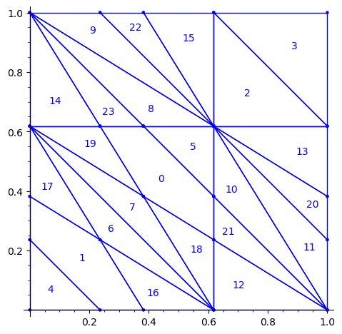
Below is a reproduction of Jang-Robinson bifurcation diagram shown in Figure 10 from arxiv:2504.10838

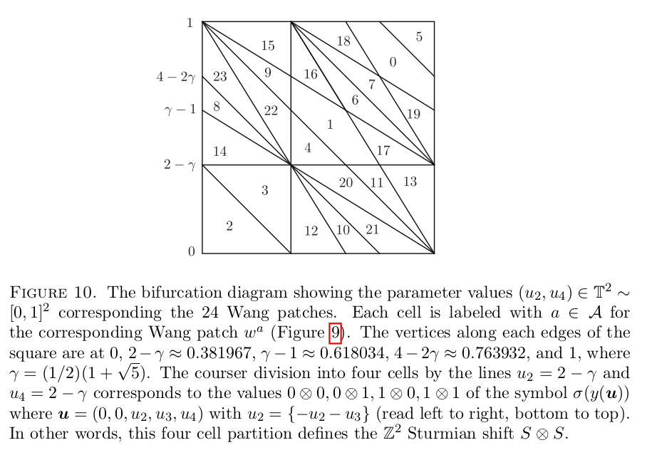
In this section, we construct this bifurcation diagram in SageMath as a polygonal partition.

sage: from slabbe import PolyhedronPartition

sage: z = polygen(QQ, 'z')
sage: K = NumberField(z**2-z-1, 'phi', embedding=RR(1.6))
sage: phi = K.gen()

sage: square = polytopes.hypercube(2,intervals = 'zero_one')
sage: P = PolyhedronPartition([square])
sage: P = P.refine_by_hyperplane([1/phi^3,-1,-1])
sage: P = P.refine_by_hyperplane([1/phi,-1,-1])
sage: P = P.refine_by_hyperplane([1,-1,-1])
sage: P = P.refine_by_hyperplane([1 + 1/phi,-1,-1])
sage: P = P.refine_by_hyperplane([1 + 1/phi^3,-1,-1])
sage: P = P.refine_by_hyperplane([1/phi,-phi,-1])
sage: P = P.refine_by_hyperplane([1,-phi,-1])
sage: P = P.refine_by_hyperplane([phi,-phi,-1])
sage: P = P.refine_by_hyperplane([1/phi^2,-1/phi,-1])
sage: P = P.refine_by_hyperplane([1/phi,-1/phi,-1])
sage: P = P.refine_by_hyperplane([1,-1/phi,-1])
sage: P = P.refine_by_hyperplane([1/phi,-1,0])
sage: P = P.refine_by_hyperplane([1/phi,0,-1])
sage: P = -P
sage: P = P.translate((1,1))
sage: #P.plot()
sage: P = P.rename_keys({0:5, 1:0, 2:18, 3:19, 4:7, 5:6, 6:16, 7:17, 8:1, 9:4, 10:15,11:9,
sage:                    12:22,13:23,14:8, 15:14,16:13,17:11,18:20,19:21,20:10, 21:12, 22:3,
sage:                    23:2})
sage: P.plot()

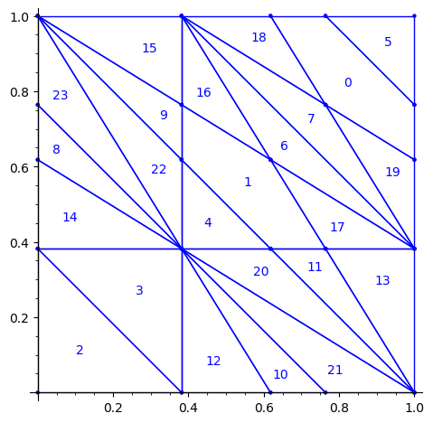
Our claim

We claim that the above bifurcation diagram from Jang-Robinson preprint is slightly wrong according to the choice of indices of the 24 Wang tiles made by Jang and Robinson and shown above. The following changes should be made in order to fix the partition:

• indices 9 and 22 should be swapped,
• indices 8 and 23 should be swapped,
• indices 11 and 20 should be swapped and
• indices 10 and 21 should be swapped.

Defining the toral translations in the internal space as PETs

We define the toral translations associated to the partition chosen by Jang-Robinson. The internal space is the 2-dimensional torus ℝ² ⁄ ℤ². It is represented as the unit square [0, 1)². On this fundamental domain, a toral translation is a polygon exchange transformation.

Note that according to their choice,

• a unit horizontal translation in the physical space corresponds to a vertical translation by (0, φ) in the internal space,
• a unit vertical translation in the physical space corresponds to a horizontal translation by (φ, 0) in the internal space,

where φ is the golden mean.

Below, we follow their convention.

sage: from slabbe import PolyhedronExchangeTransformation as PET

sage: base = diagonal_matrix((1,1))
sage: R0e1 = PET.toral_translation(base, vector((0,phi)))
sage: R0e2 = PET.toral_translation(base, vector((phi,0)))

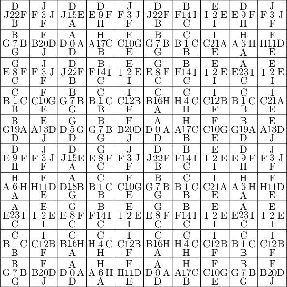
We compute a 10 × 10 pattern obtained by coding the orbit of some starting point under the ℤ²-action R₀.

sage: from slabbe.coding_of_PETs import PETsCoding

sage: coding_R0_P = PETsCoding((R0e1,R0e2), P)
sage: pattern = coding_R0_P.pattern((.3,.4), (10,10))
sage: pattern = WangTiling(pattern, T0)
sage: pattern.tikz()

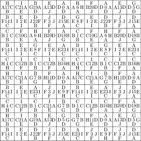
We observe that this pattern is not valid !!!

Let's fix the partition

We claim that the above pattern is wrong because something is wrong in the labelling of the atoms in the partition proposed by Jang and Robinson for the 24 Wang tiles encoding Penrose tilings.

Below, we fix the partition by swapping labels 8 and 23, 9 and 22, 11 and 20, 10 and 21:

sage: d = {i:i for i in range(24)}
sage: d.update({8:23, 23:8, 9:22, 22:9, 11:20, 20:11, 10:21, 21:10})
sage: P1 = P.rename_keys(d)
sage: P1.plot()

We compute a 10 × 10 pattern out of this updated partition P₁:

sage: coding_R0_P1 = PETsCoding((R0e1,R0e2), P1)
sage: pattern = coding_R0_P1.pattern((.3,.4), (10,10))
sage: pattern = WangTiling(pattern, T0)
sage: pattern.tikz()

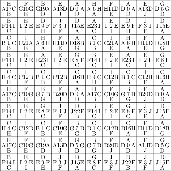
We observe that this pattern is valid !!!

Understanding the issue using edge label partitions

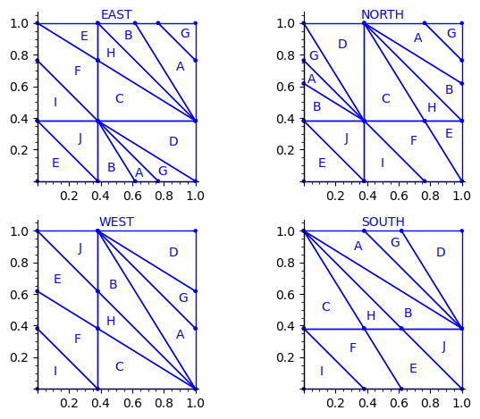
Let us try to understand the fix in terms of the Wang tiles east, north, west and south edge labels partitions induced by the original partition.

Indeed, since each atom of the partition corresponds to a Wang tile, we can deduce a partition of the unit square for the east labels (and respectively for the north, west and south labels) by merging two atoms in the partition if their east edge label is the same.

sage: def edge_label_partitions(partition, tiles):
....:     EAST = partition.merge_atoms({i:tiles[i][0] for i in range(24)})
....:     NORTH = partition.merge_atoms({i:tiles[i][1] for i in range(24)})
....:     WEST = partition.merge_atoms({i:tiles[i][2] for i in range(24)})
....:     SOUTH = partition.merge_atoms({i:tiles[i][3] for i in range(24)})
....:     return EAST, NORTH, WEST, SOUTH
sage: def draw_edge_label_partitions(partition, tiles):
....:     EAST, NORTH, WEST, SOUTH = edge_label_partitions(partition, tiles)
....:     L = [EAST.plot() + text('EAST', (.5,1.05)),
....:          NORTH.plot() + text('NORTH', (.5,1.05)),
....:          WEST.plot() + text('WEST', (.5,1.05)),
....:          SOUTH.plot() + text('SOUTH', (.5,1.05))]
....:     return graphics_array(L, nrows=2)

This is what we get using the partition proposed by Jang and Robinson for the 24 Wang tiles encoding Penrose tilings:

sage: draw_edge_label_partitions(P, T0)

Here are some observations which are normal:

• partitions NORTH and EAST are symmetric under a reflexion by the positive diagonal (remember that the tile set is symmetric under the positive diagonal)
• partitions WEST and SOUTH are symmetric under a reflexion by the positive diagonal (remember that the tile set is symmetric under the positive diagonal)

Here are some observations which are not normal:

• partitions WEST and EAST do not give the same area to the same index (in a Wang tiling, the frequency of a EAST label should be equal to the frequency of the same WEST label)
• partitions SOUTH and NORTH do not give the same area to the same index (in a Wang tiling, the frequency of a NORTH label should be equal to the frequency of the same SOUTH label)
• partitions EAST and WEST are not a translate of one another (idealy a horizontal translate)
• partitions SOUTH and NORTH are not a translate of one another (idealy a vertical translate)

Another indication that something may be wrong is:

• atoms B, H, E, J, A, G are not convex in the torus

This is not a necessity. Atoms are not convex in the Markov partition associated to Jeandel-Rao tilings [2]. But they are convex for the Ammann set of 16 Wang tiles and their generalization to metallic mean numbers made in [3,4]. Since Penrose tilings are closely related to Ammann A2 tilings, we may also expect to have simple convex atoms in each of the four edge label partitions.

Here is the area of each atom in each of the four partitions. We observe that only atoms C and D have the same area in each of the four partitions.

sage: def table_of_area_of_atom_in_east_north_west_south_partitions(partition, tiles):
....:     columns = []
....:     labels = 'ABCDEFGHIJ'
....:     EAST, NORTH, WEST, SOUTH = edge_label_partitions(partition, tiles)
....:     for partition in [EAST, NORTH, WEST, SOUTH]:
....:         d = partition.volume_dict()
....:         column = [d[a] for a in labels]
....:         columns.append(column)
....:     header_row = ['EAST', 'NORTH', 'WEST', 'SOUTH']
....:     return table(columns=columns, header_row=header_row, header_column=['']+list(labels))

sage: table_of_area_of_atom_in_east_north_west_south_partitions(P, T0)
    │ EAST             NORTH            WEST             SOUTH
├───┼────────────────┼────────────────┼────────────────┼────────────────┤
  A │ 15/2*phi - 12    15/2*phi - 12    phi - 3/2        phi - 3/2
  B │ phi - 3/2        phi - 3/2        15/2*phi - 12    15/2*phi - 12
  C │ phi - 3/2        phi - 3/2        phi - 3/2        phi - 3/2
  D │ phi - 3/2        phi - 3/2        phi - 3/2        phi - 3/2
  E │ phi - 3/2        phi - 3/2        -11/2*phi + 9    -11/2*phi + 9
  F │ -11/2*phi + 9    -11/2*phi + 9    phi - 3/2        phi - 3/2
  G │ -8*phi + 13      -8*phi + 13      -3/2*phi + 5/2   -3/2*phi + 5/2
  H │ -3/2*phi + 5/2   -3/2*phi + 5/2   -8*phi + 13      -8*phi + 13
  I │ 5*phi - 8        5*phi - 8        -3/2*phi + 5/2   -3/2*phi + 5/2
  J │ -3/2*phi + 5/2   -3/2*phi + 5/2   5*phi - 8        5*phi - 8

But, we observe that we can fix the partitions if we assume that the atoms C and D in the four partitions are correct. There is a unique translation sending atoms C,D in the partition WEST to the atoms C and D in the partition EAST. That translation should send the partition WEST exactly on EAST. Similarly for SOUTH and NORTH. This suggest a way to fix atoms B, H, E, J, A, G in the partition.

Fixed Edge labels partitions

Using the fixed partition, here is what we get.

sage: P1.plot()

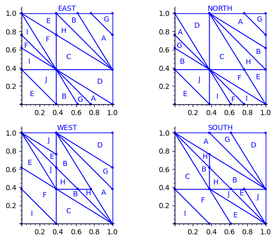
sage: draw_edge_label_partitions(P1, T0)

Now it looks good! As for the partitions associated to the metallic mean Wang tiles, the four partitions are isometric copies of the other ones (under toral translation or reflection).

sage: table_of_area_of_atom_in_east_north_west_south_partitions(P1, T0)
    │ EAST             NORTH            WEST             SOUTH
├───┼────────────────┼────────────────┼────────────────┼────────────────┤
  A │ phi - 3/2        phi - 3/2        phi - 3/2        phi - 3/2
  B │ phi - 3/2        phi - 3/2        phi - 3/2        phi - 3/2
  C │ phi - 3/2        phi - 3/2        phi - 3/2        phi - 3/2
  D │ phi - 3/2        phi - 3/2        phi - 3/2        phi - 3/2
  E │ phi - 3/2        phi - 3/2        phi - 3/2        phi - 3/2
  F │ phi - 3/2        phi - 3/2        phi - 3/2        phi - 3/2
  G │ -3/2*phi + 5/2   -3/2*phi + 5/2   -3/2*phi + 5/2   -3/2*phi + 5/2
  H │ -3/2*phi + 5/2   -3/2*phi + 5/2   -3/2*phi + 5/2   -3/2*phi + 5/2
  I │ -3/2*phi + 5/2   -3/2*phi + 5/2   -3/2*phi + 5/2   -3/2*phi + 5/2
  J │ -3/2*phi + 5/2   -3/2*phi + 5/2   -3/2*phi + 5/2   -3/2*phi + 5/2

sage: (phi-3/2).n(), (-3/2*phi + 5/2).n()
(0.118033988749895, 0.0729490168751576)

Labels A, B, C, D, E and F all have the same frequency of φ − (3)/(2) ≈ 0.118.

Labels G, H, I and J all have the same frequency of  − (3)/(2)φ + (5)/(2) ≈ 0.0729.

We check that frequencies sum to 1:

sage: 6 * (phi-3/2) + 4 * (-3/2*phi + 5/2)
1

Proposed partition for the encoding of the Penrose tilings into 24 Wang tiles

As done with the Markov partition associated to Jeandel-Rao aperiodic tilings, and for the Markov partition associated to the family of metallic mean Wang tiles, I think it is more natural to associate horizontal (vertical) translations in the internal space with horizontal (vertical) translations in the physical space. This way, the brain is less mixed up and the projections in the physical space π and in the internal space π_int of the cut and project scheme are defined more naturally. This way the internal space and physical space can even be identified: this is the root of the do-it-yourself tutorial allowing the construction of Jeandel-Rao tilings [5]. See also my Habilitation à diriger des recherches written in English during Spring 2025 for more information [6].

First, we flip the partition P₁ by the positive diagonal. This exchanges the role of x and y axis.

sage: P2 = P1.apply_linear_map(matrix(2, [0,1,1,0]))
sage: P2.plot()

This allows to define the ℤ²-action R₁ on the torus with horizontal and vertical translations for e₁ and e₂ respectively:

sage: base = diagonal_matrix((1,1))
sage: R1e1 = PET.toral_translation(base, vector((1/phi,0)))
sage: R1e2 = PET.toral_translation(base, vector((0,1/phi)))

Then, we rotate the partition. This changes the origin of the partition. This change may be optional, but it makes the partition look closer to the partitions already studied in [2,3,4]. It simplifies the explanation of any relation between them (and there is one, see below!).

sage: P3 = R1e1(P2)
sage: P3 = R1e2(P3)
sage: P3.plot()

We observe that the partition P₃ associated to the 24 Wang tiles encoding Penrose tiling is a refinement of the partition associated to the 16 Ammann tiles (see Figure 15 in [4] as the 16 Ammann tiles are equivalent to the n-th metallic mean Wang tiles when n = 1).

We compute a 10 × 10 pattern obtained by coding the orbit of some starting point under the ℤ²-action R₁ using partition P₃.

sage: from slabbe.coding_of_PETs import PETsCoding

sage: coding_R1_P3 = PETsCoding((R1e1,R1e2), P3)
sage: pattern = coding_R1_P3.pattern((.3,.4), (10,10))
sage: pattern = WangTiling(pattern, T0)
sage: pattern.tikz()

We are happy to see that the pattern is still valid after all the changes we have made!

sage: draw_edge_label_partitions(P3, T0)

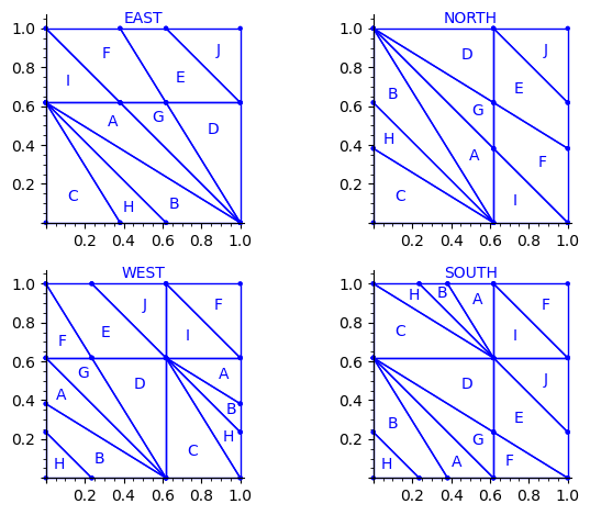
We observe that the EAST, NORTH, WEST and SOUTH partitions are a refinement of the EAST, NORTH, WEST and SOUTH partitions associated to the Ammann tiles partition (see Figure 15 in [4]).

The difference between the Ammann EAST and 24 Wang tiles Penrose EAST partition is the addition of two closed geodesics of slope -1 on the 2-torus passing through the origin and through the vertex (0, φ^− 1).

It is possible that there is a clever way of including this information into the labels of the Wang tiles as we have done it for the family of metallic mean Wang tiles. Possibly, we need to use 4-dimension vectors for the tile labels instead of 3-dimensional integer vectors. This remains an open question.

Wang tiles deduced from the partition and ℤ²-action

We check that the Wang tiles computed from the partition P₃ and ℤ²-action R₁ is the original set of 24 Wang tiles defined by Jang and Robinson.

See Proposition 8.1 in [2].

sage: T = coding_R1_P3.to_wang_tiles()
sage: T.tikz()

sage: T.is_equivalent(T0, certificate=True)
(True,
 {'3': 'D',
  '0': 'A',
  '6': 'G',
  '1': 'B',
  '7': 'H',
  '2': 'C',
  '8': 'I',
  '4': 'E',
  '5': 'F',
  '9': 'J'},
 {'3': 'D',
  '0': 'A',
  '6': 'G',
  '1': 'B',
  '7': 'H',
  '2': 'C',
  '8': 'I',
  '4': 'E',
  '5': 'F',
  '9': 'J'},
 Substitution 2d: {0: [[0]], 1: [[1]], 2: [[2]], 3: [[3]], 4: [[4]], 5:
 [[5]], 6: [[6]], 7: [[7]], 8: [[8]], 9: [[9]], 10: [[10]], 11: [[11]], 12:
 [[12]], 13: [[13]], 14: [[14]], 15: [[15]], 16: [[16]], 17: [[17]], 18: [[18]],
 19: [[19]], 20: [[20]], 21: [[21]], 22: [[22]], 23: [[23]]})