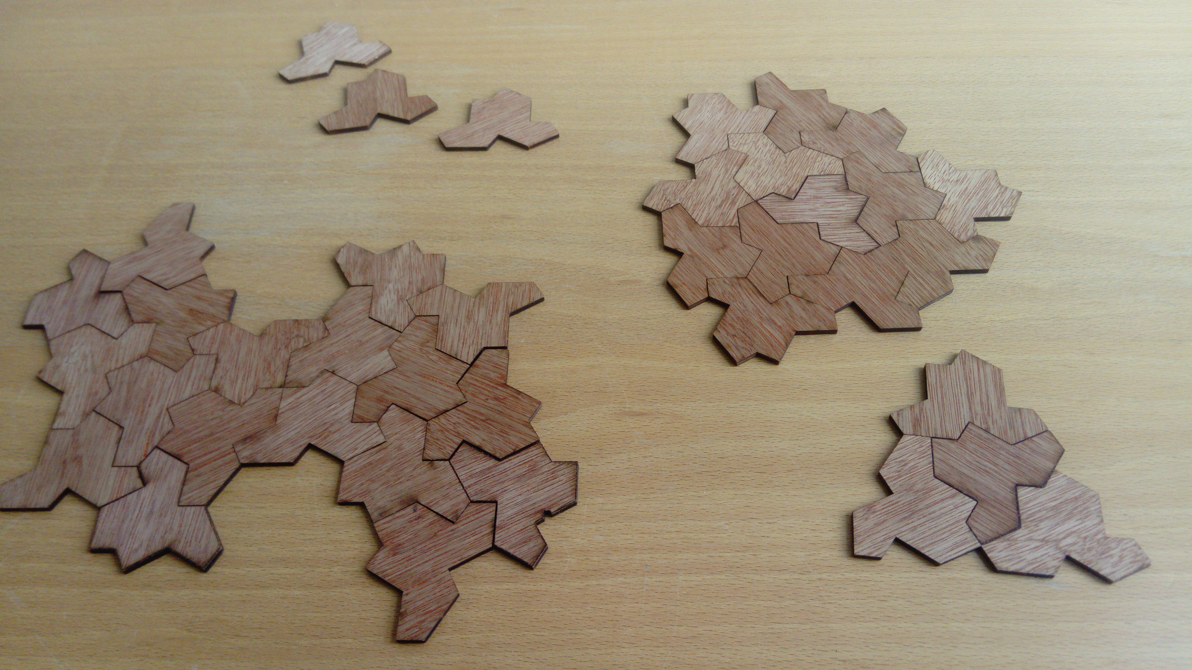
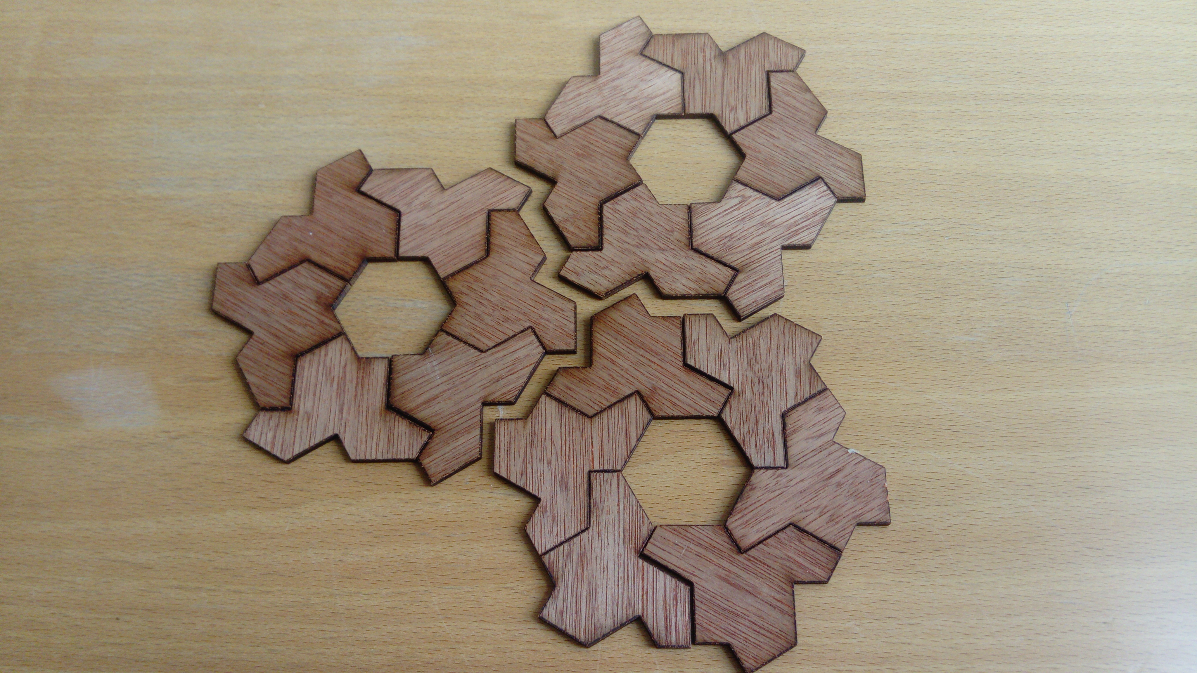
In 2015, Emmanuel Jeandel and Michael Rao discovered a very nice set of 11 Wang tiles which can be encoded geometrically into the following set of 11 geometrical shapes:
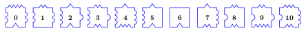
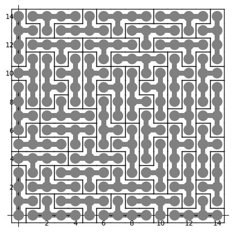
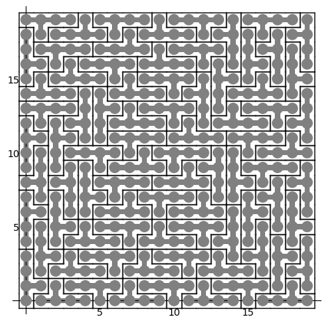
Jeandel and Rao proved that you may tile the plane with infinitely many translated copies of these tiles, but never periodically:
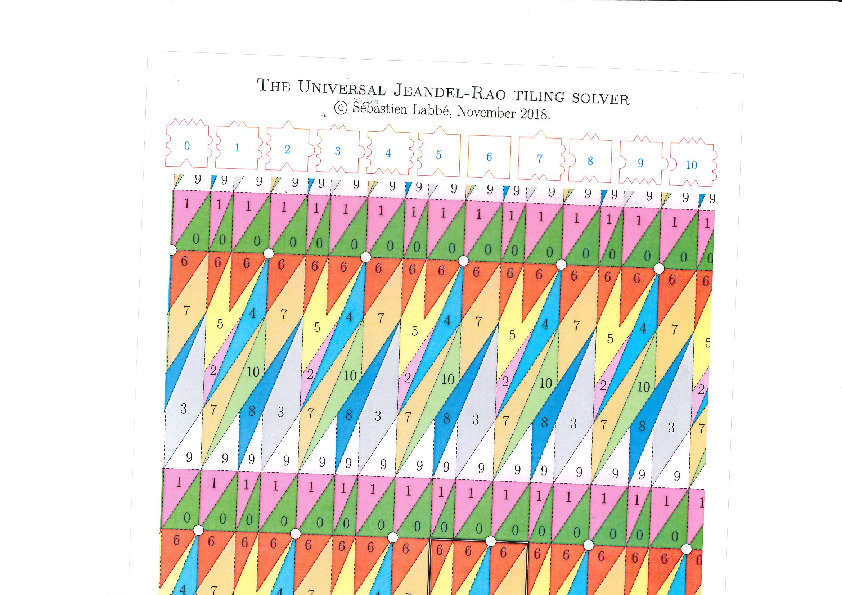
There is an easy way to construct Jeandel-Rao tilings from a well-chosen polygonal partition of the plane.
This is the polygonal partition:
A lattice, represented below by the set of intersection of two perpendicular set of gridlines, is placed at a random position on top of the partition:
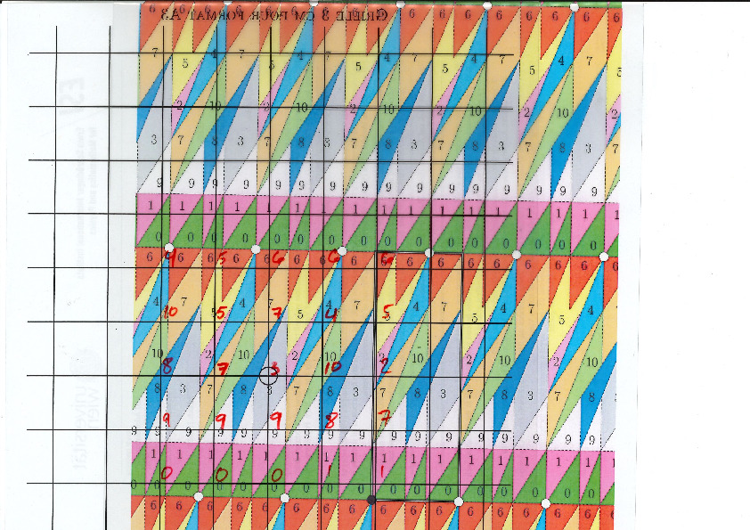
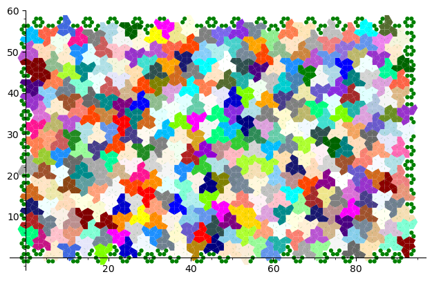
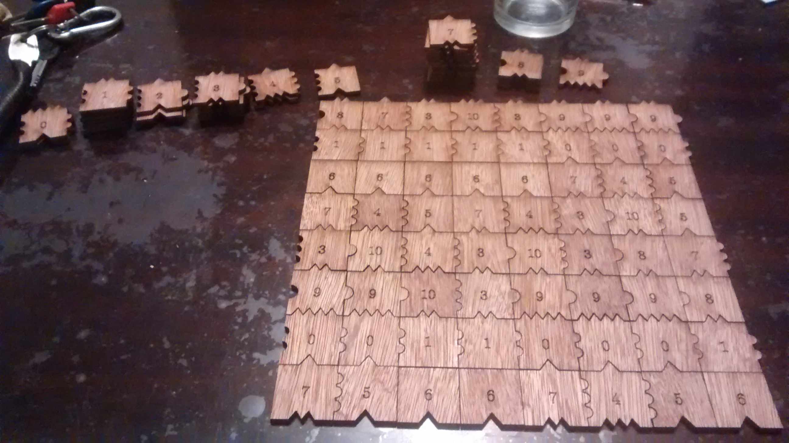
Each point of the lattice can be associated to an index from 0 to 10 according to which polygon of the partition it falls in. This defines a configuration of indices associated to each integer coordinate:
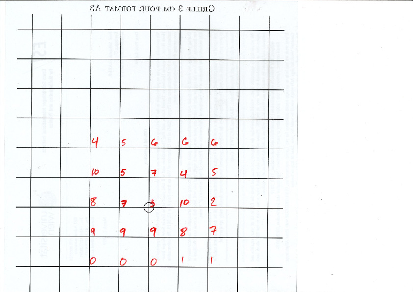
This procedure can be done all the way up to infinity. The chosen placement of the lattice defines a valid tiling of the plane with Jeandel-Rao tiles!

Since the size of the fundamental domain of the polygonal partition is irrational (width is golden mean, height is golden mean + 3, while the distance between two parallel gridlines is 1 unit), the generated configuration must be non-periodic.
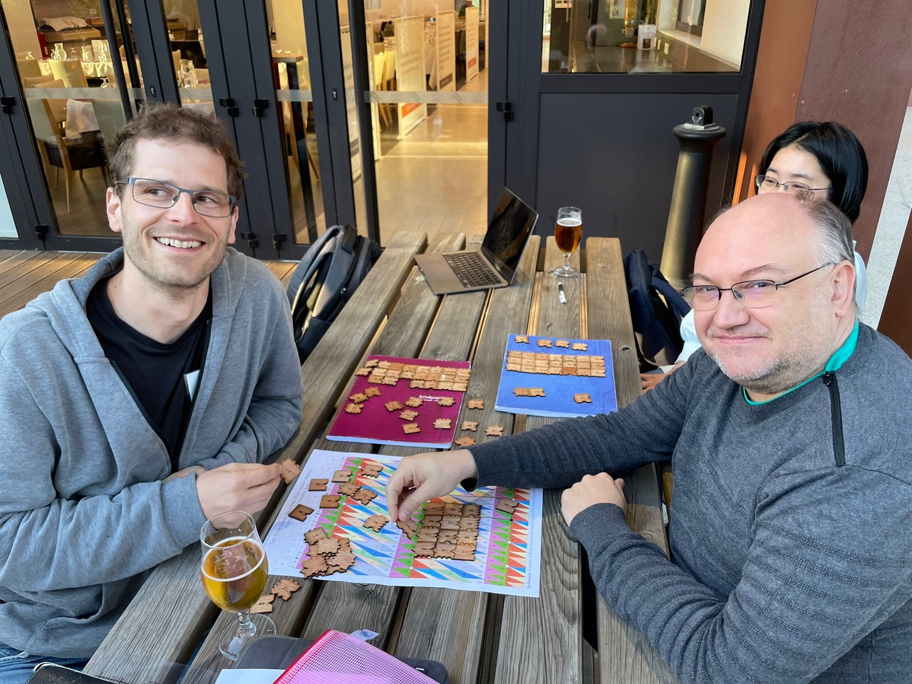
It was a pleasure for me to do illustrate this to Emmanuel Jeandel during the workshop Multidimensional symbolic dynamics and lattice models of quasicrystals at CIRM in April 2024 in Marseille.
Do it yourself
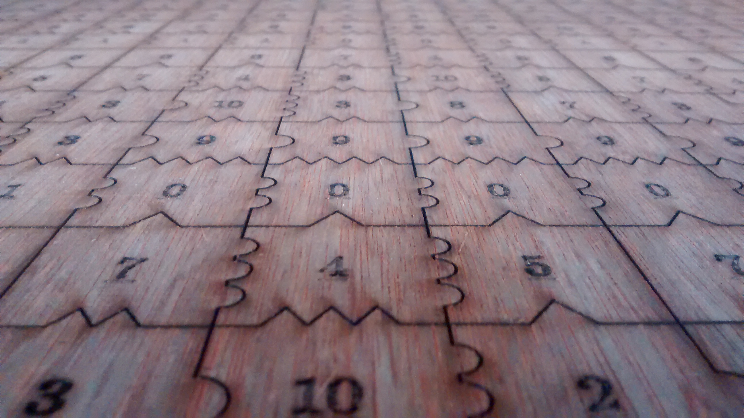
Here are the files allowing to reproduce this experiment:
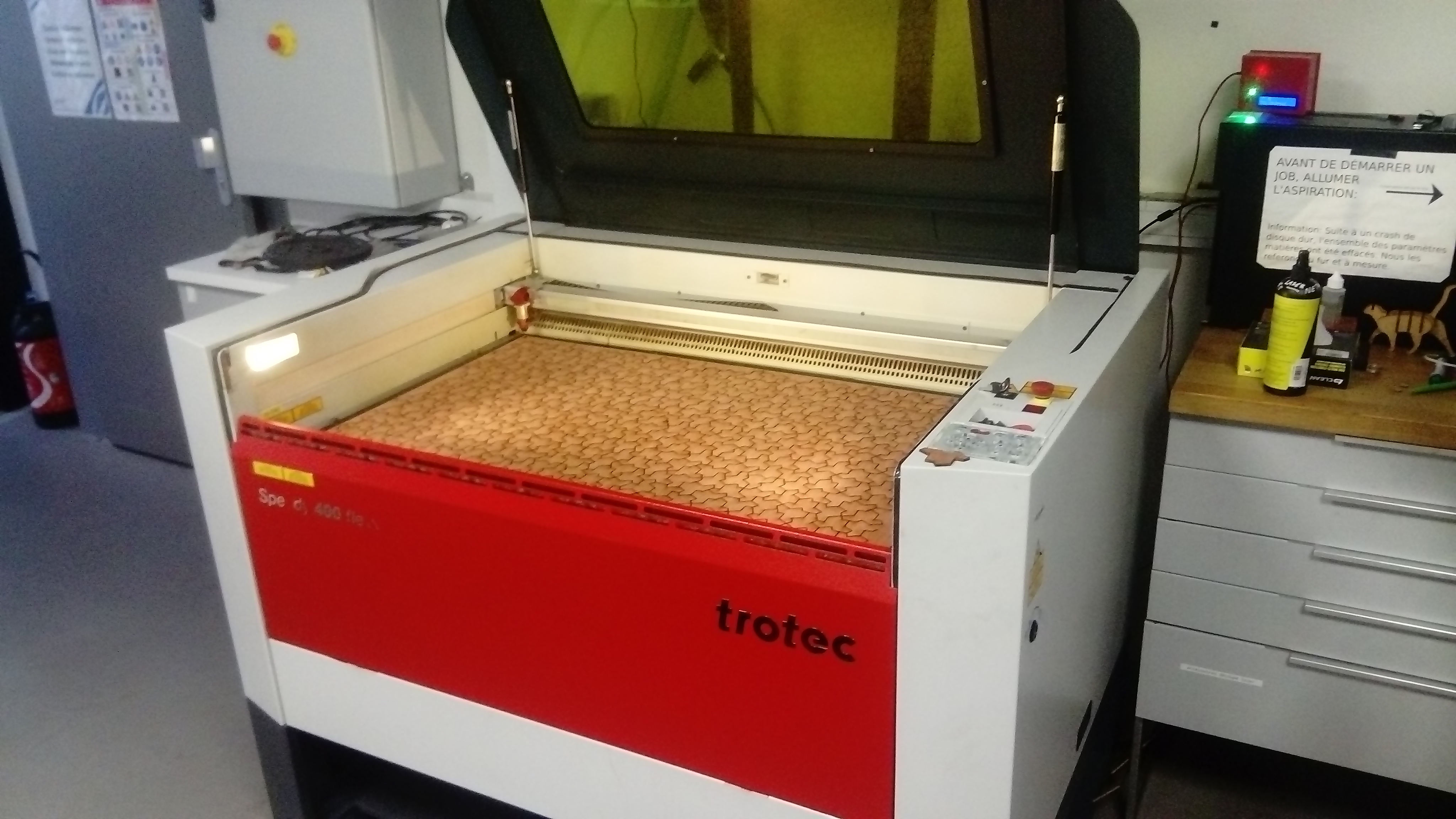
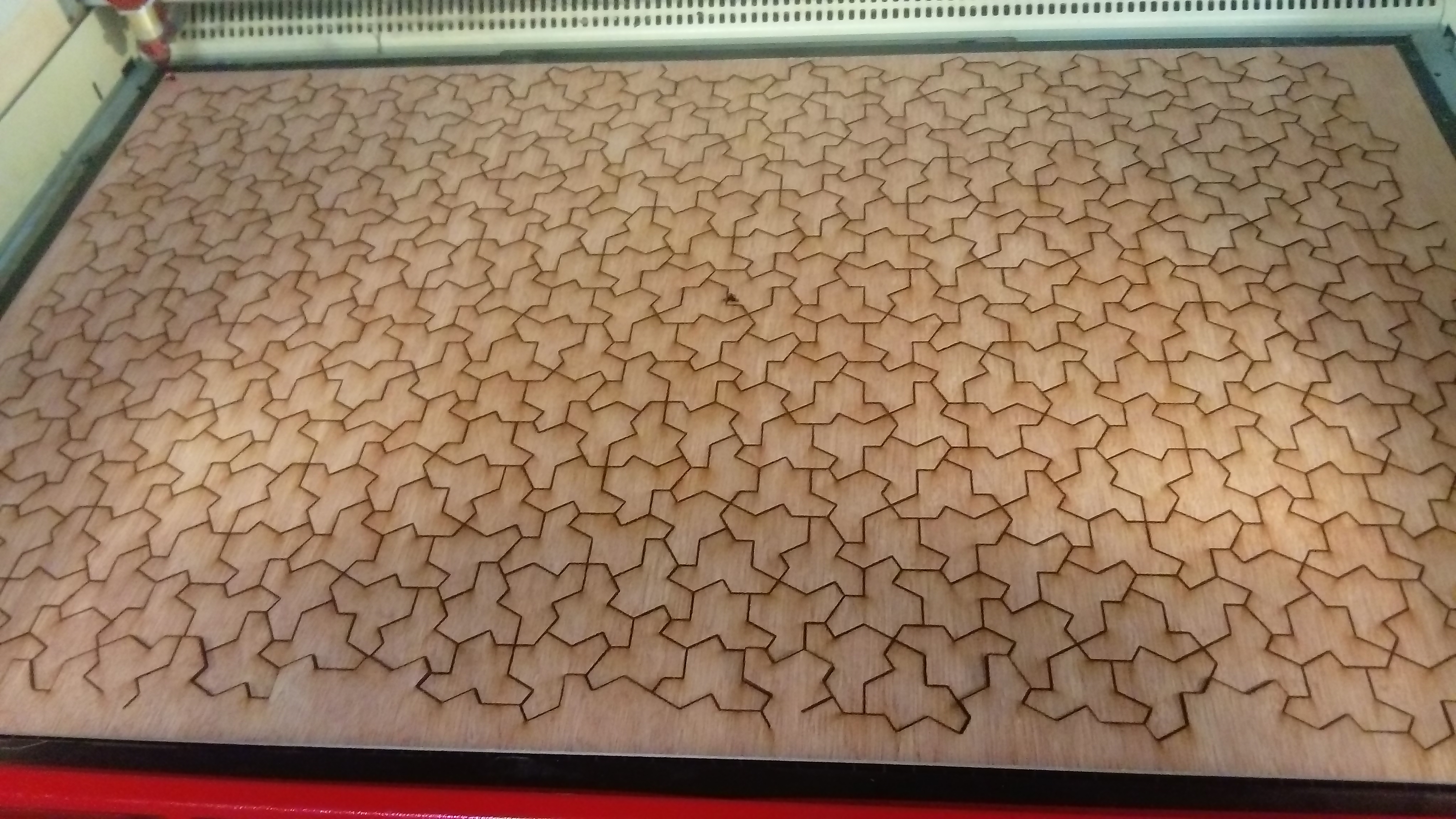
- A 33 x 19 rectangular valid patch of 627 tiles to use to cut a 1 meter x 60 cm wooden flat sheet (in svg format for laser cutting, pieces should have a side length of exactly 3 cm after the operation)
- The polygonal partition to be printed on a A3 paper (1 unit = 3 cm)
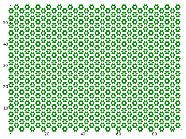
- The lattice \(\mathbb{Z}^2\) represented by gridlines 3cm apart to be printed on A4 paper (1 unit = 3 cm)
- The one-page Jeandel-Rao tiling solver tutorial
Alternate files for laser cutting the tiles
I first cut those tiles in August 2018 before a conference in Durham with the help of David Renault. We made more of them in June 2019. Each time David does some changes to the file that I provide to him with InkScape. Here are three alternate files for laser cutting the tiles.
Frequency of tiles
The frequency of tiles in a Jeandel-Rao tilings is computed below from the relative area in the associated polygonal partition. Tile #2 is the least frequent (around 2.55%) while tile #7 is the most frequent (around 15%):
sage: from slabbe.arXiv_1903_06137 import jeandel_rao_wang_shift_partition
sage: P0 = jeandel_rao_wang_shift_partition()
sage: V = P0.volume()
sage: tile_frequency = {a:v/V for (a,v) in P0.volume_dict().items()}
sage: rows = [(a, tile_frequency[a], tile_frequency[a].n(digits=3)) for a in range(11)]
sage: table(rows, header_row=['tile', 'frequency', 'frequency (numerical approx)'])
  tile   frequency           frequency (numerical approx)
├──────┼───────────────────┼──────────────────────────────┤
  0      -1/22*phi + 2/11    0.108
  1      -1/22*phi + 2/11    0.108
  2      9/22*phi - 7/11     0.0255
  3      -1/22*phi + 2/11    0.108
  4      2/11*phi - 5/22     0.0669
  5      -5/11*phi + 9/11    0.0828
  6      -1/22*phi + 2/11    0.108
  7      -3/11*phi + 13/22   0.150
  8      2/11*phi - 5/22     0.0669
  9      -1/22*phi + 2/11    0.108
  10     2/11*phi - 5/22     0.0669
When I construct a bag of 50 tiles of the Jeandel-Rao tiles, I follow the above tile frequencies. It yields:
sage: [(tile_frequency[a]*52).n(digits=3) for a in range(11)]
[5.63, 5.63, 1.33, 5.63, 3.48, 4.30, 5.63, 7.78, 3.48, 5.63, 3.48]
sage: [round(a) for a in _]
[6, 6, 1, 6, 3, 4, 6, 8, 3, 6, 3]
sage: sum(_)
52
Discussion
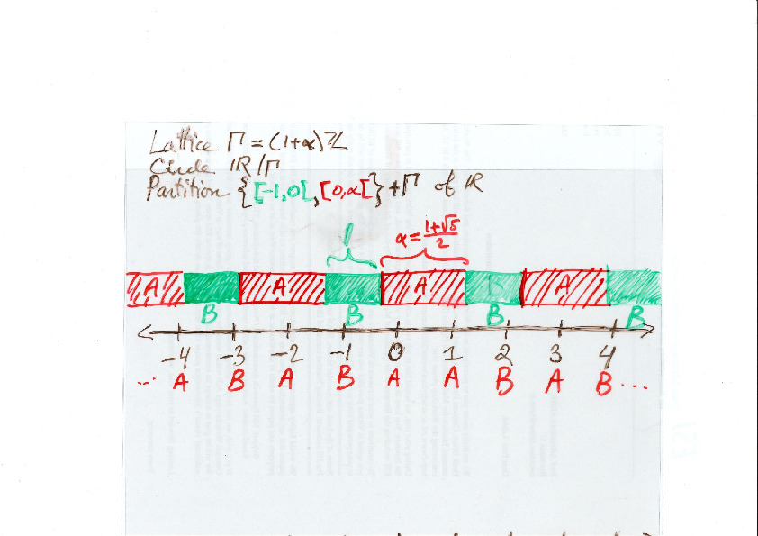
The construction of valid tilings with Jeandel-Rao tiles from a polygonal partition is a generalization of a well-known phenomenon in one dimension, namely, the fact that Sturmian sequences of complexity \(n+1\) are coded by irrational rotations. For example, here is an easy way to construct Sturmian sequences using a partition of the line into two intervals of different lengths. Similarly as above, every point from a set of equidistanced points is coded by letter A or B according to which of the two intervals it falls in.
The question that one may ask is whether all Jeandel-Rao tilings can be constructed from such a starting point in the partition. For Sturmian sequences, the answer is yes and the starting point can be described using the Ostrowski numeration system and the continued fraction expansion of the slope defined from the ratio of frequencies of the letters in the sequence. In one dimension, the proof is thus based on the desubstitution of Sturmian sequences on the one hand, and the Rauzy induction of irrational rotations on the other hand.
The same approach can be performed for Jeandel-Rao tilings using 2-dimensional desubstitution of Wang tilings and 2-dimensional Rauzy induction of toral \(\mathbb{Z}^2\)-rotations. Surprisingly, the two totally different methods applied on two completely different objects lead to the same sequence of eventually periodic 2-dimensional substitutions. Thus, every Jeandel-Rao tiling that can be desubstituted indefinitely can be constructed from the coding of some starting point in the polygonal partition.
Unfortunately, not all Jeandel-Rao tilings can be desubstituted indefinitely because of the existence of a horizontal fault line breaking the substitutive structure. Some configuration have a biinfinite horizontal row of the same tile labeled 0 in them. This allows to slide the lower half of configuration along the fault line and the configuration remains valid. A conjecture is that the remaining configurations are rare (of probability zero according to any shift-invariant probability measure). More precisely, I believe that all of the problematic ones can be described by a pair of starting points on the bottom segment of the polygonal partition. During the sabbatical year of Casey Mann and Jennifer Mcloud-Mann in Bordeaux in 2019-2020, we tried hard to prove that conjecture without success. It seems to be a difficult problem. Instead we described the nonexpansive directions in Jeandel-Rao tilings which reminds of the behavior of Penrose tilings with respect to Conway worms, their resolutions and essential holes (annulus of tiles which can be completed uniquely outside of the annulus, but not inside).
Aperiodic tilings related to the Metallic mean
The structure of Penrose aperiodic tilings, Jeandel-Rao aperiodic tilings and the new aperiodic hat monotile are all related to the golden mean. Do all aperiodic tilings need to be related to the golden ratio? What other numbers can be achieved?
During the conference at CIRM, I presented my newest result split into two parts: for every positive integer \(n\), there exists an aperiodic set of \((n+3)^2\) Wang tiles whose tiling structure is associated to the \(n\)-th metallic mean number, that is, the positive root of the polynomial \(x^2-nx-1\). This new discovery extends the knowledge we have on aperiodic tilings beyond the omnipresent golden ratio. The talk was recorded on youtube and the written notes are available here.
Jean-René Chazottes et Marc Monticelli
During the conference at CIRM, I met Jean-René Chazottes and Marc Monticelli. They made me know about their interactive online books, the outreach mathemarium website and its online experiments. Also, the Open-Fabrik-Maths fablab in Nice, including some experiments involving aperiodic Wang tilings.
]]>