Wooden laser-cut Jeandel-Rao tiles

07 septembre 2018 | Catégories: sage, slabbe spkg, math, découpe laser | View Comments

I have been working on Jeandel-Rao tiles lately.

Before the conference Model Sets and Aperiodic Order held in Durham UK (Sep 3-7 2018), I thought it would be a good idea to bring some real tiles at the conference. So I first decided of some conventions to represent the above tiles as topologically closed disk basically using the representation of integers in base 1:

With these shapes, I created a 33 x 19 patch. With 3cm on each side, the patch takes 99cm x 57cm just within the capacity of the laser cut machine (1m x 60 cm):

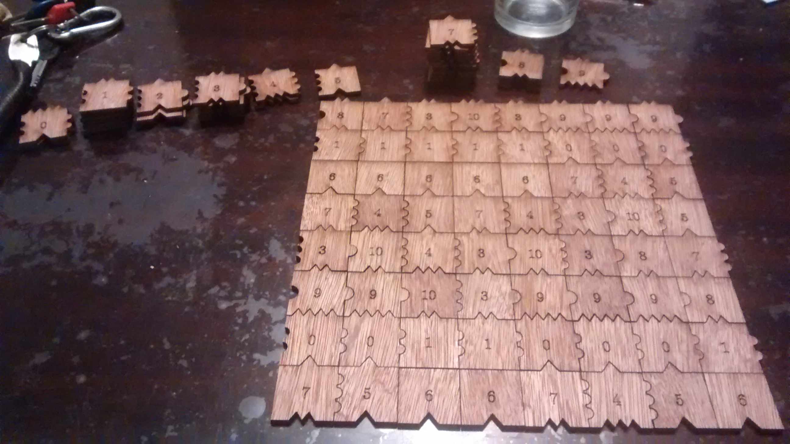
With the help of David Renault from LaBRI, we went at Coh@bit, the FabLab of Bordeaux University and we laser cut two 3mm thick plywood for a total of 1282 Wang tiles. This is the result:

One may recreate the 33 x 19 tiling as follows (note that I am using Cartesian-like coordinates, so the first list data[0] actually is the first column from bottom to top):

sage: data = [[10, 4, 6, 1, 3, 3, 7, 0, 9, 7, 2, 6, 1, 3, 8, 7, 0, 9, 7],
....:  [4, 5, 6, 1, 8, 10, 4, 0, 9, 3, 8, 7, 0, 9, 7, 5, 0, 9, 3],
....:  [3, 7, 6, 1, 7, 2, 5, 0, 9, 8, 7, 5, 0, 9, 3, 7, 0, 9, 10],
....:  [10, 4, 6, 1, 3, 8, 7, 0, 9, 7, 5, 6, 1, 8, 10, 4, 0, 9, 3],
....:  [2, 5, 6, 1, 8, 7, 5, 0, 9, 3, 7, 6, 1, 7, 2, 5, 0, 9, 8],
....:  [8, 7, 6, 1, 7, 5, 6, 1, 8, 10, 4, 6, 1, 3, 8, 7, 0, 9, 7],
....:  [7, 5, 6, 1, 3, 7, 6, 1, 7, 2, 5, 6, 1, 8, 7, 5, 0, 9, 3],
....:  [3, 7, 6, 1, 10, 4, 6, 1, 3, 8, 7, 6, 1, 7, 5, 6, 1, 8, 10],
....:  [10, 4, 6, 1, 3, 3, 7, 0, 9, 7, 5, 6, 1, 3, 7, 6, 1, 7, 2],
....:  [2, 5, 6, 1, 8, 10, 4, 0, 9, 3, 7, 6, 1, 10, 4, 6, 1, 3, 8],
....:  [8, 7, 6, 1, 7, 5, 5, 0, 9, 10, 4, 6, 1, 3, 3, 7, 0, 9, 7],
....:  [7, 5, 6, 1, 3, 7, 6, 1, 10, 4, 5, 6, 1, 8, 10, 4, 0, 9, 3],
....:  [3, 7, 6, 1, 10, 4, 6, 1, 3, 3, 7, 6, 1, 7, 2, 5, 0, 9, 8],
....:  [10, 4, 6, 1, 3, 3, 7, 0, 9, 10, 4, 6, 1, 3, 8, 7, 0, 9, 7],
....:  [4, 5, 6, 1, 8, 10, 4, 0, 9, 3, 3, 7, 0, 9, 7, 5, 0, 9, 3],
....:  [3, 7, 6, 1, 7, 2, 5, 0, 9, 8, 10, 4, 0, 9, 3, 7, 0, 9, 10],
....:  [10, 4, 6, 1, 3, 8, 7, 0, 9, 7, 5, 5, 0, 9, 10, 4, 0, 9, 3],
....:  [2, 5, 6, 1, 8, 7, 5, 0, 9, 3, 7, 6, 1, 10, 4, 5, 0, 9, 8],
....:  [8, 7, 6, 1, 7, 5, 6, 1, 8, 10, 4, 6, 1, 3, 3, 7, 0, 9, 7],
....:  [7, 5, 6, 1, 3, 7, 6, 1, 7, 2, 5, 6, 1, 8, 10, 4, 0, 9, 3],
....:  [3, 7, 6, 1, 10, 4, 6, 1, 3, 8, 7, 6, 1, 7, 2, 5, 0, 9, 8],
....:  [10, 4, 6, 1, 3, 3, 7, 0, 9, 7, 2, 6, 1, 3, 8, 7, 0, 9, 7],
....:  [4, 5, 6, 1, 8, 10, 4, 0, 9, 3, 8, 7, 0, 9, 7, 5, 0, 9, 3],
....:  [3, 7, 6, 1, 7, 2, 5, 0, 9, 8, 7, 5, 0, 9, 3, 7, 0, 9, 10],
....:  [10, 4, 6, 1, 3, 8, 7, 0, 9, 7, 5, 6, 1, 8, 10, 4, 0, 9, 3],
....:  [3, 3, 7, 0, 9, 7, 5, 0, 9, 3, 7, 6, 1, 7, 2, 5, 0, 9, 8],
....:  [8, 10, 4, 0, 9, 3, 7, 0, 9, 10, 4, 6, 1, 3, 8, 7, 0, 9, 7],
....:  [7, 5, 5, 0, 9, 10, 4, 0, 9, 3, 3, 7, 0, 9, 7, 5, 0, 9, 3],
....:  [3, 7, 6, 1, 10, 4, 5, 0, 9, 8, 10, 4, 0, 9, 3, 7, 0, 9, 10],
....:  [10, 4, 6, 1, 3, 3, 7, 0, 9, 7, 5, 5, 0, 9, 10, 4, 0, 9, 3],
....:  [2, 5, 6, 1, 8, 10, 4, 0, 9, 3, 7, 6, 1, 10, 4, 5, 0, 9, 8],
....:  [8, 7, 6, 1, 7, 5, 5, 0, 9, 10, 4, 6, 1, 3, 3, 7, 0, 9, 7],
....:  [7, 5, 6, 1, 3, 7, 6, 1, 10, 4, 5, 6, 1, 8, 10, 4, 0, 9, 3]]

The above patch have been chosen among 1000 other randomly generated as the closest to the asymptotic frequencies of the tiles in Jeandel-Rao tilings (or at least in the minimal subshift that I describe in the preprint):

sage: from collections import Counter
sage: c = Counter(flatten(data))
sage: tile_count = [c[i] for i in range(11)]

The asymptotic frequencies:

sage: phi = golden_ratio.n()
sage: Linv = [2*phi + 6, 2*phi + 6, 18*phi + 10, 2*phi + 6, 8*phi + 2,
....:      5*phi + 4, 2*phi + 6, 12/5*phi + 14/5, 8*phi + 2,
....:      2*phi + 6, 8*phi + 2]
sage: perfect_proportions = vector([1/a for a in Linv])

Comparison of the number of tiles of each type with the expected frequency:

sage: header_row = ['tile id', 'Asymptotic frequency', 'Expected nb of copies',
....:               'Nb copies in the 33x19 patch']
sage: columns = [range(11), perfect_proportions, vector(perfect_proportions)*33*19, tile_count]
sage: table(columns=columns, header_row=header_row)
  tile id   Asymptotic frequency   Expected nb of copies   Nb copies in the 33x19 patch
+---------+----------------------+-----------------------+------------------------------+
  0         0.108271182329550      67.8860313206280        67
  1         0.108271182329550      67.8860313206280        65
  2         0.0255593590340479     16.0257181143480        16
  3         0.108271182329550      67.8860313206280        71
  4         0.0669152706817991     41.9558747174880        42
  5         0.0827118232955023     51.8603132062800        51
  6         0.108271182329550      67.8860313206280        65
  7         0.149627093977301      93.8161879237680        95
  8         0.0669152706817991     41.9558747174880        44
  9         0.108271182329550      67.8860313206280        67
  10        0.0669152706817991     41.9558747174880        44

I brought the \(33\times19=641\) tiles at the conference and offered to the first 7 persons to find a \(7\times 7\) tiling the opportunity to keep the 49 tiles they used. 49 is a good number since the frequency of the lowest tile (with id 2) is about 2% which allows to have at least one copy of each tile in a subset of 49 tiles allowing a solution.

A natural question to ask is how many such \(7\times 7\) tilings does there exist? With ticket #25125 that was merged in Sage 8.3 this Spring, it is possible to enumerate and count solutions in parallel with Knuth dancing links algorithm. After the installation of the Sage Optional package slabbe (sage -pip install slabbe), one may compute that there are 152244 solutions.

sage: from slabbe import WangTileSet
sage: tiles = [(2,4,2,1), (2,2,2,0), (1,1,3,1), (1,2,3,2), (3,1,3,3),
....: (0,1,3,1), (0,0,0,1), (3,1,0,2), (0,2,1,2), (1,2,1,4), (3,3,1,2)]
sage: T0 = WangTileSet(tiles)
sage: T0_solver = T0.solver(7,7)
sage: %time T0_solver.number_of_solutions(ncpus=8)
CPU times: user 16 ms, sys: 82.3 ms, total: 98.3 ms
Wall time: 388 ms
152244

One may also get the list of all solutions and print one of them:

sage: %time L = T0_solver.all_solutions(); print(len(L))
152244
CPU times: user 6.46 s, sys: 344 ms, total: 6.8 s
Wall time: 6.82 s
sage: L[0]
A wang tiling of a 7 x 7 rectangle
sage: L[0].table()  # warning: the output is in Cartesian-like coordinates
[[1, 8, 10, 4, 5, 0, 9],
 [1, 7, 2, 5, 6, 1, 8],
 [1, 3, 8, 7, 6, 1, 7],
 [0, 9, 7, 5, 6, 1, 3],
 [0, 9, 3, 7, 6, 1, 8],
 [1, 8, 10, 4, 6, 1, 7],
 [1, 7, 2, 2, 6, 1, 3]]

This is the number of distinct sets of 49 tiles which admits a 7x7 solution:

sage: from collections import Counter
sage: def count_tiles(tiling):
....:     C = Counter(flatten(tiling.table()))
....:     return tuple(C.get(a,0) for a in range(11))
sage: Lfreq = map(count_tiles, L)
sage: Lfreq_count = Counter(Lfreq)
sage: len(Lfreq_count)
83258

Number of other solutions with the same set of 49 tiles:

sage: Counter(Lfreq_count.values())
Counter({1: 49076, 2: 19849, 3: 6313, 4: 3664, 6: 1410, 5: 1341, 7: 705, 8:
293, 9: 159, 14: 116, 10: 104, 12: 97, 18: 44, 11: 26, 15: 24, 13: 10, 17: 8,
22: 6, 32: 6, 16: 3, 28: 2, 19: 1, 21: 1})

How the number of \(k\times k\)-solutions grows for k from 0 to 9:

sage: [T0.solver(k,k).number_of_solutions() for k in range(10)]
[0, 11, 85, 444, 1723, 9172, 50638, 152244, 262019, 1641695]

Unfortunately, most of those \(k\times k\)-solutions are not extendable to a tiling of the whole plane. Indeed the number of \(k\times k\) patches in the language of the minimal aperiodic subshift that I am able to describe and which is a proper subset of Jeandel-Rao tilings seems, according to some heuristic, to be something like:

[1, 11, 49, 108, 184, 268, 367, 483]

I do not share my (ugly) code for this computation yet, as I will rather share clean code soon when times come. So among the 152244 about only 483 (0.32%) of them are prolongable into a uniformly recurrent tiling of the plane.

Sébastien Labbé

Wooden laser-cut Jeandel-Rao tiles