Introduction to Python/SageMath
27 juin 2023 | Catégories: sage, math | View CommentsOn Wednesday June 28th, 2023, I give short a Introduction to Python/SageMath as an online course organized by Pierre-Guy Plamondon in Mathematical Summer in Paris (MSP23) on WorkAdventure. Below is the material that will be presented or suggested.
Exercises:
- Install and open a Jupyter notebook and do the User Interface Tour in the help menu.
- Programming with Python. Here is a list of Jupyter notebooks to learn programming in Python: ProgrammingExercises.zip or ProgrammingExercises.tar.xz
- Reproduce the computations made by BuzzFeedNews in a github repository of your choice, for instance about the fentanyl and cocaine overdose deaths (2018) or about The Tennis Racket (2016).
- Solve some problems from the Project Euler. Project Euler contains more than 500 exercises that have to be solved with a computer
- Reproduce one or more images from the matplotlib library.
- Download the book Mathematical Computation with Sage by Paul Zimmermann et al. about the SageMath open source software. Reproduce the computations made in a section of your choice in the book.
- Visit https://ask.sagemath.org/questions/ and try to reproduce some of the best answers to questions of interest for you.
- Choose a section of your choice in the SageMath very large Reference Manual and reproduce the computations made in it.
When working on the above, two principles applies:
- Once you finished solving a notebook or a problem on Project Euler on your own you need to explain your solution to at least one other person (who has already solved the same notebook or problem).
- Once you reproduced the computation made by BuzzFeedNews, matplotlib image or some computation, you need to present and explain it to at least one other person.
Supplementary material:
- Experimenting with Dynamical systems in SageMath: DynamicalSystemExercices.zip
- Some more notebooks and exercices from this course given by Vincent Delecroix at AIMS in Rwanda (2016).
Découpe laser du chapeau, tuile apériodique découverte récemment
25 mai 2023 | Catégories: sage, slabbe spkg, math, découpe laser | View CommentsLe chapeau est une tuile apériodique découverte par David Smith, Joseph Samuel Myers, Craig S. Kaplan, et Chaim Goodman-Strauss le 20 mars 2023. Suite à un exposé donné le 26 mars au National Museum of Mathematics, la nouvelle s'est vite répandue. En effet, cette découverte a été mentionnée les jours suivants dans des blogues puis dans Le New York Times le 28 mars, Le Monde le 29 mars, puis The Guardian et QuantaMagazine le 4 avril. Un vidéo de 20 minutes, réalisé par Passe-Science et publié début le 3 mai, explique le résultat et son contexte.
Déjà des articles proposant des résultats plus approfondis sur la tuile par des experts du domaine sont parus sur arXiv en mai 2023. Ils interprêtent les pavages comme des coupes et projection de réseaux de dimension supérieure. Le deuxième propose même une partition de la fenêtre de l'espace interne, un peu comme pour les pavages de Jeandel-Rao, à la différence qu'ici la partition a des bords fractales ce qui est pour moi une grande surprise.
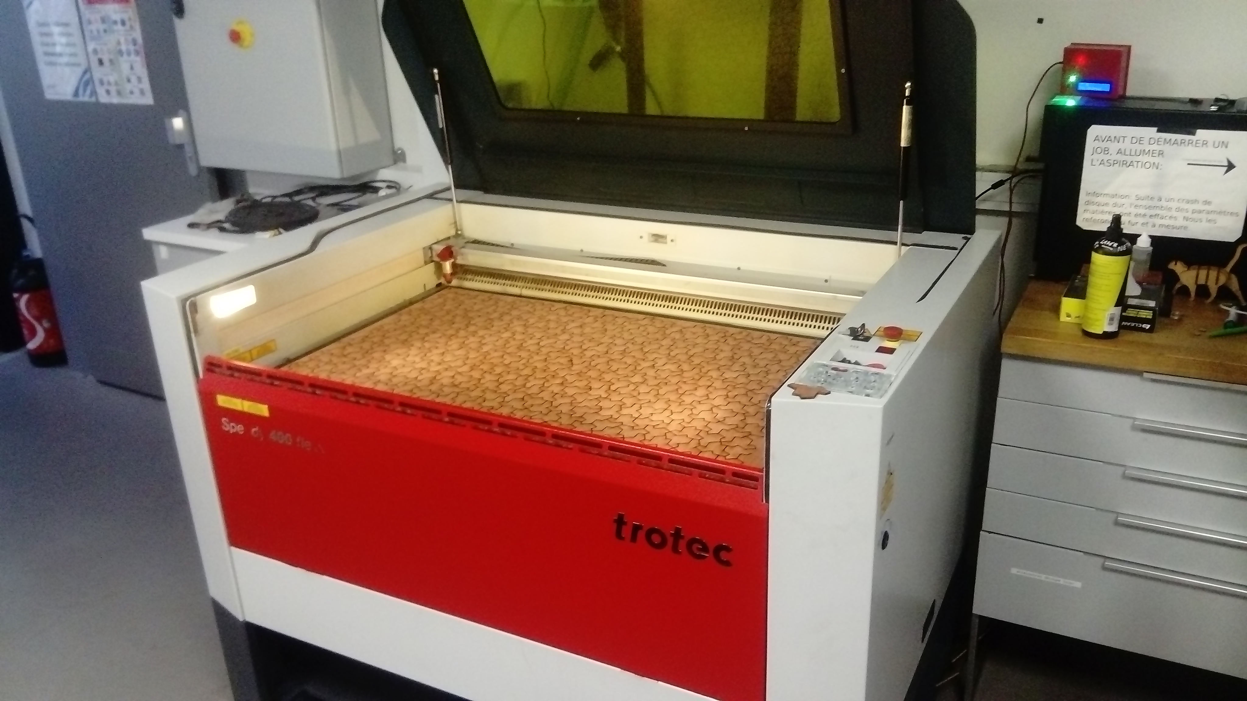
Comme je faisais une intervention dans l'école de mon garçon à Bègles le 3 mai et au Lycée Kastler de Talence le 4 mai, j'ai réalisé un projet de découpe laser sur la tuile apériodique afin de partager cette récente découverte.
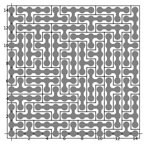
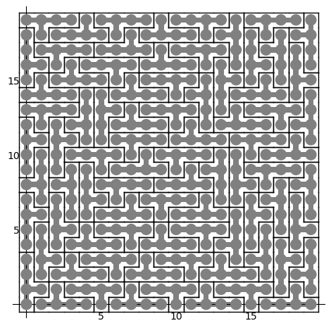
La première question était de construire un pavage d'un rectangle assez grand avec la pièce apériodique. Pour ce faire, j'ai ajouté un nouveau module dans mon package optionel au logiciel SageMath.
Le module réalise une réduction à une instance du problème de la couverture universelle, qui peut être résolu dans SageMath en utilisant l'algorithme des liens dansants de Donald Knuth, les solveurs SAT ou les programmes d'optimisation linéaire (solveur MILP). Le code utilise le système de coordonnées défini dans le fichier validate/kitegrid.pdf qui se trouve dans le code source associé à l'article.
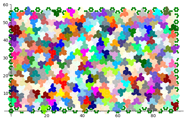
Voici un exemple de construction d'un pavage avec la tuile apériodique. Le calcul est fait dans le logiciel SageMath muni de la version de développement de mon package optionnel slabbe qui peut être installé avec la commande sage -pip install slabbe. Ici, j'utilise le solveur SAT Glucose, développé au LaBRI. On peut installer glucose dans SageMath avec la commande sage -i glucose.
sage: from slabbe.aperiodic_monotile import MonotileSolver
sage: s = MonotileSolver(16, 17)
sage: G = s.draw_one_solution(solver='glucose')
sage: G.save('solution_16x17.png')
sage: G
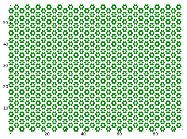
Dans la manière de résoudre la question ci-haut, le problème est représenté par un problème de couverture exacte qui consiste à recouvrir exactement les entiers de 1 à n avec des sous-ensembles choisis dans une liste de sous-ensembles déterminés. Ici, on représente l'espace à recouvrir de manière discrète en comptant 6 points du plan par hexagone (un point pour chaque kite contenu dans un hexagone). Rappelons que la pièce Chapeau qui nous intéresse est formée d'une union d'exactement 8 de ces kites.
sage: s.plot_domain()
Ensuite, on construit une matrice de 0 et de 1 avec autant de colonnes que de points ci-haut (16 * 17 * 2 * 6 = 3264) et autant de lignes qu'il y a de copies isométriques de la pièce intersectant le domaine. Pour chaque copie de la pièce, une ligne dans la matrice contient des 1 exactement dans les colonnes associées aux kites occupés par la pièce.
sage: s.the_dlx_solver()
Dancing links solver for 3264 columns and 7116 rows
Le calcul ci-haut qui a construit la matrice (sparse) indique qu'il y a 7116 copies isométriques de la pièce qui intersectent (complètement ou partiellement) le domaine. Quand on voudra dessiner une solution, on ignorera les pièces incomplètes.
On peut maintenant résoudre le problème.
sage: s = MonotileSolver(8,8)
sage: %time L = s.one_solution()   # l'algo des liens dansants de Knuth est utilisé par défaut
CPU times: user 798 ms, sys: 32.2 ms, total: 830 ms
Wall time: 1min 20s
Le contenu d'une solution est une liste de nombres indiquant les lignes de la matrice de 0/1 à considérer pour former une solution. C'est-à-dire que la sous-matrice restreinte aux lignes données comporte exactement un 1 dans chaque colonne:
sage: L
[81,
 85,
 125,
 128,
 ...
 1772,
 1783,
 1794,
 1815]
Ici, il se trouve que les solveurs SAT sont plus efficaces que l'algo des liens dansants pour trouver une solution:
sage: %time L = s.one_solution(solver='glucose')
CPU times: user 326 ms, sys: 16.1 ms, total: 342 ms
Wall time: 526 ms
sage: %time L = s.one_solution(solver='kissat')
CPU times: user 335 ms, sys: 3.64 ms, total: 339 ms
Wall time: 461 ms
En effet, Glucose se comporte plutôt bien pour résoudre des problèmes de pavages du plan lorsqu'il existe une solution. Mais lorsqu'il n'y a pas de solution, l'algo des liens dansants de Knuth est parfois mieux. Aussi, l'algo des liens dansants de Knuth est très efficace pour énumérer toutes les solutions.
Le solveur Kissat a été ajouté dans SageMath par moi-même comme package optionnel cette année suite à une discussion avec Laurent Simon au café du LaBRI. On peut installer le solveur kissat dans SageMath avec la commande sage -i kissat.
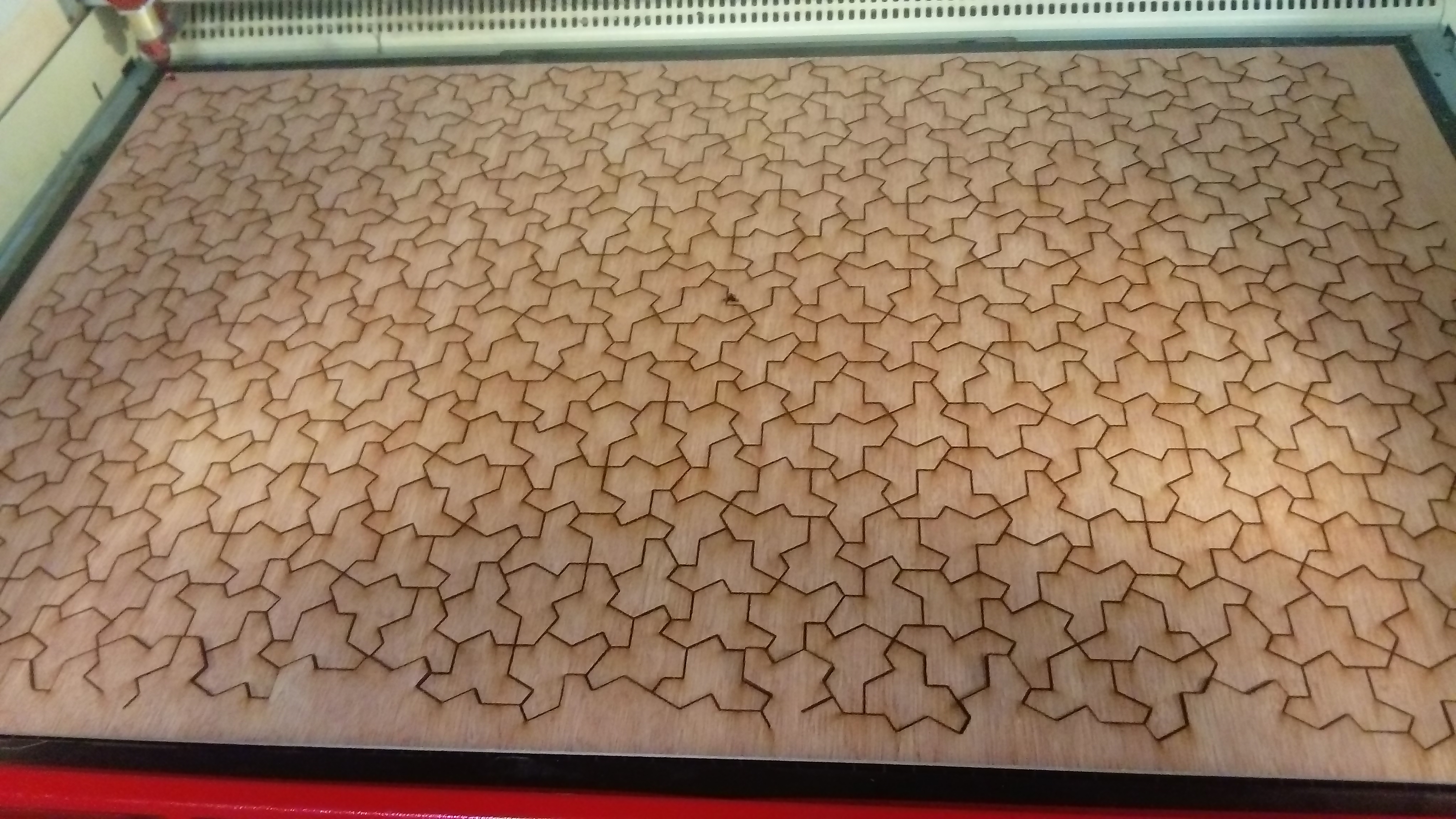
Ici on extrait le contour des pièces d'une solution (tel que chaque arête est dessinée une seule fois afin d'éviter que la découpeuse laser passe deux fois par chaque arête ce qui peut endommager ou brûler le bord des pièces en bois) et on crée un fichier pdf ou svg. Je choisis une taille de 16 double-hexagones horizontalement et 17 verticalement, car cela crée un fichier qui correspond à une taille de 1m x 60cm. C'est la taille de la découpeuse laser à notre disposition:
sage: s = MonotileSolver(16, 17)
sage: tikz = s.one_solution_tikz(solver='glucose')
sage: tikz.pdf('solution_16x17.pdf')
sage: tikz.svg('solution_16x17.svg')     # or
Avec l'aide de David Renault, mon collègue du LaBRI qui enseigne à l'ENSEIRB et qui m'a déjà accompagné dans la réalisation de projets de découpe laser, nous avons découpé le fichier ci-haut le jeudi 27 avril au EirLab, l'atelier de fabrication numérique (FabLab) de l'ENSEIRB-MATMECA:
Comme toujours, il faut quelque peu modifier le fichier svg dans Inkscape avant de lancer la découpe laser. Voici le fichier modifié juste avant la découpe.
Maintenant, on peut s'amuser avec les pièces:
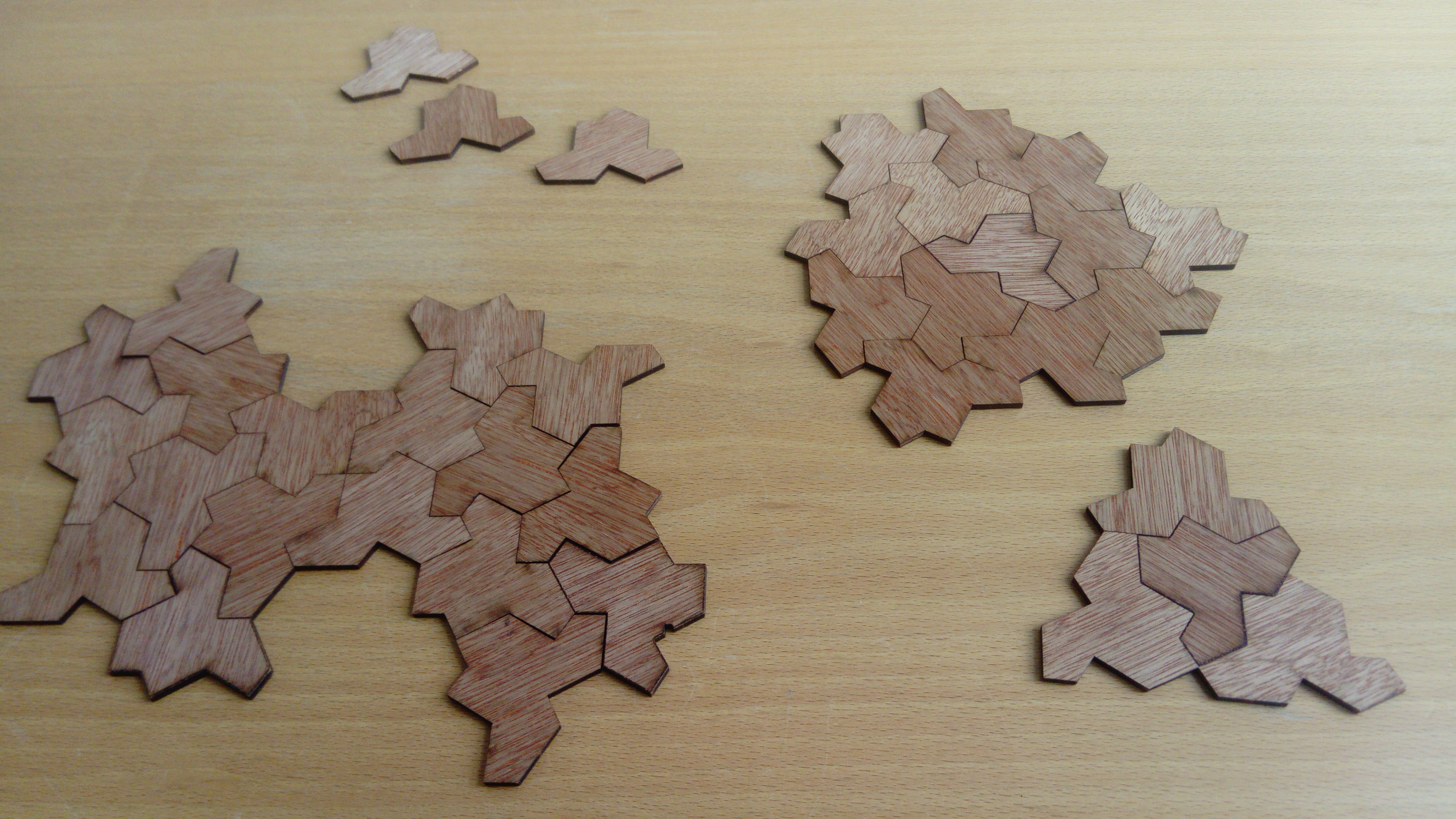
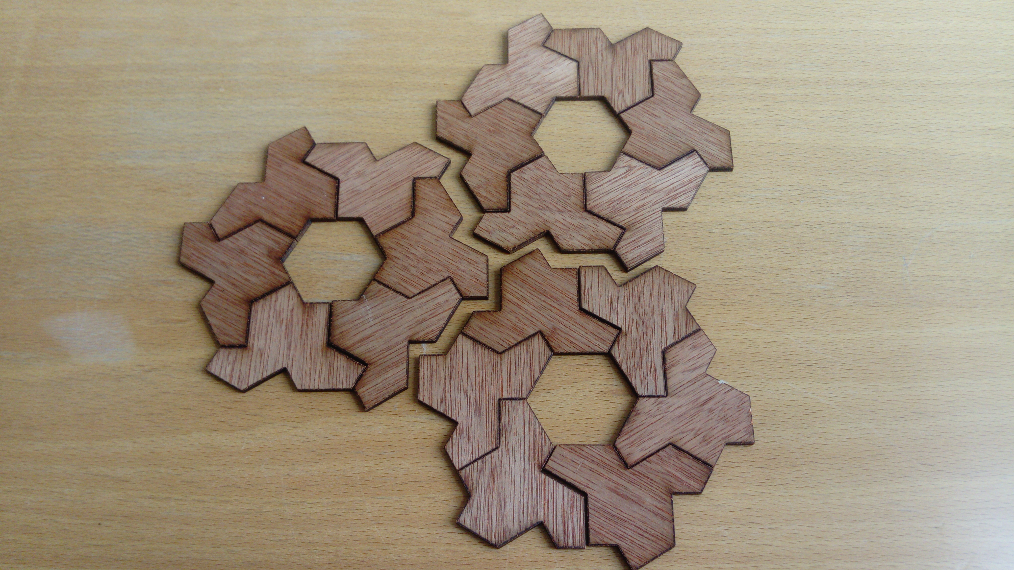
Avec mes garçons, nous avons trouvé une forme intéressante qui recouvre le plan périodiquement à l'exception d'un trou hexagonal. Il se trouve que la même forme peut-être créée de deux façons différentes: sur l'image ci-bas la forme à droite est la globalement la même, mais elle n'est pas obtenue de la même façon que celle en haut à gauche. Pourtant, toutes deux ont le même contour extérieur et le même trou hexagonal.
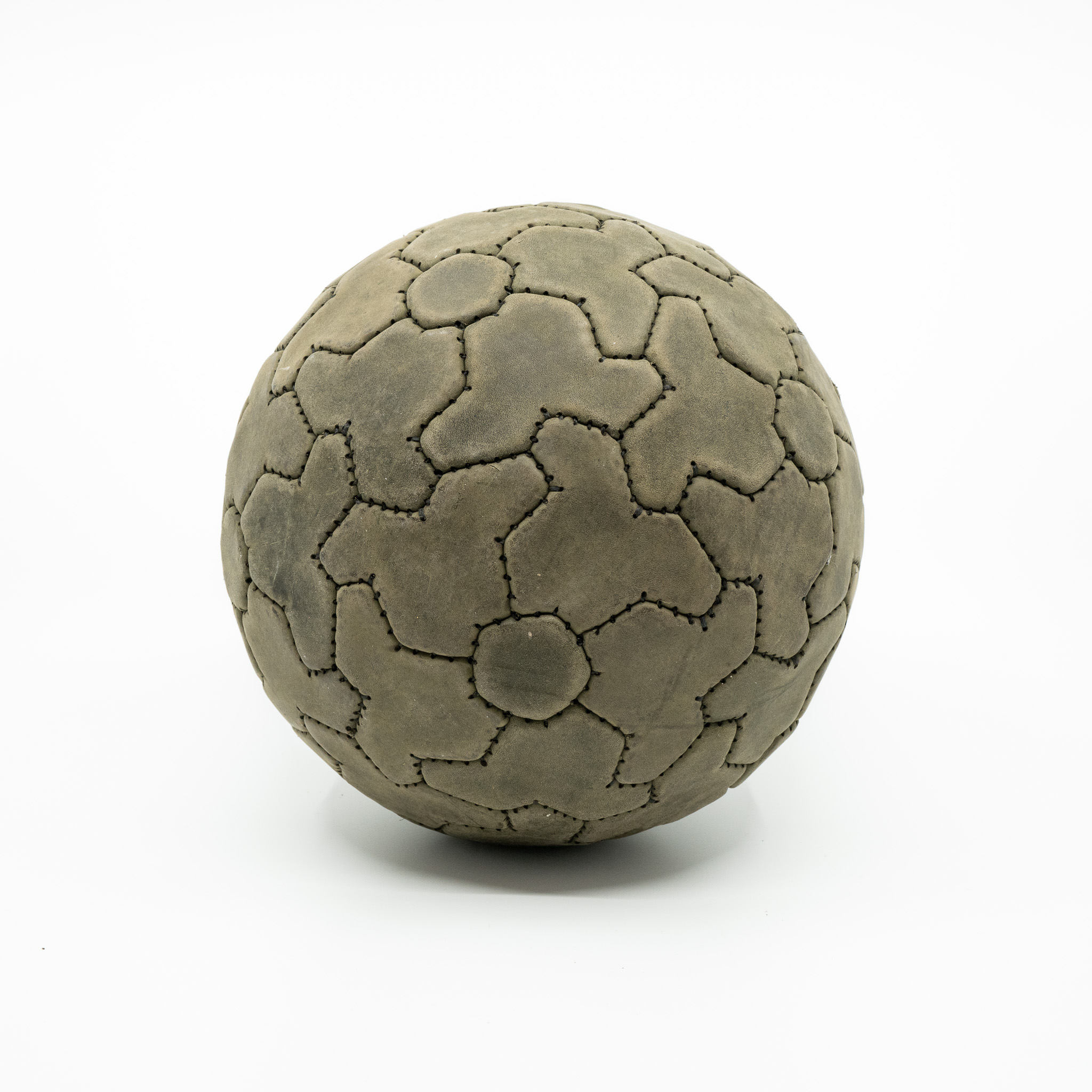
Cette observation, déjà faite par d'autres, a mené au recouvrement d'une sphère avec la pièce et un trou pentagonal:
Using Glucose SAT solver to find a tiling of a rectangle by polyominoes
27 mai 2021 | Mise à jour: 20 juin 2022 | Catégories: sage, math | View CommentsIn his Dancing links article, Donald Knuth considered the problem of packing 45 Y pentaminoes into a 15 x 15 square. We can redo this computation in SageMath using some implementation of his dancing links algorithm.
Dancing links takes 1.24 seconds to find a solution:
sage: from sage.combinat.tiling import Polyomino, TilingSolver
sage: y = Polyomino([(0,0),(1,0),(2,0),(3,0),(2,1)])
sage: T = TilingSolver([y], box=(15, 15), reusable=True, reflection=True)
sage: %time solution = next(T.solve())
CPU times: user 1.23 s, sys: 11.9 ms, total: 1.24 s
Wall time: 1.24 s
The first solution found is:
sage: sum(T.row_to_polyomino(row_number).show2d() for row_number in solution)
What is nice about dancing links algorithm is that it can list all solutions to a problem. For example, it takes less than 3 minutes to find all solutions of tiling a 15 x 15 rectangle with the Y polyomino:
sage: %time T.number_of_solutions()
CPU times: user 2min 46s, sys: 3.46 ms, total: 2min 46s
Wall time: 2min 46s
1696
It takes more time (38s) to find a first solution of a larger 20 x 20 rectangle:
sage: T = TilingSolver([y], box=(20,20), reusable=True, reflection=True)
sage: %time solution = next(T.solve())
CPU times: user 38.2 s, sys: 7.88 ms, total: 38.2 s
Wall time: 38.2 s
The polyomino tiling problem is reduced to an instance of the universal cover problem which is represented by a sparse matrix of 0 and 1:
sage: dlx = T.dlx_solver()
sage: dlx
Dancing links solver for 400 columns and 2584 rows
We observe that finding a solution to this problem takes the same amount of time. This is normal since it is exactly what is used behind the scene when calling next(T.solve()) above:
sage: %time sol = dlx.one_solution(ncpus=1)
CPU times: user 38.6 s, sys: 48 ms, total: 38.6 s
Wall time: 38.5 s
One way to improve the time it takes it to split the problem into parts and use many processors to work on each subproblems. Here a random column is used to split the problem which may affect the time it takes. Sometimes a good column is chosen and it works great as below, but sometimes it does not:
sage: %time sol = dlx.one_solution(ncpus=2)
CPU times: user 941 µs, sys: 32 ms, total: 32.9 ms
Wall time: 1.41 s
The reduction from dancing links instance to SAT instance #29338 and to MILP instance #29955 was merged into SageMath 9.2 during the last year. A discussion with Franco Saliola motivated me to implement these translations since he was also searching for faster way to solve dancing links problems. Indeed some problems are solved faster with other kind of solver, so it is good to make some comparisons between solvers.
Therefore, with a recent enough version of SageMath, we can now try to find a tiling with other kinds of solvers. Following my experience with tilings by Wang tiles, I know that Glucose SAT solver is quite efficient to solve tilings of the plane. This is why I test this one below. Glucose is now an optional package to SageMath which can be installed with:
sage -i glucose
Update (June 20th, 2022): It seems sage -i glucose no longer works. The new procedure is to use ./configure --enable-glucose when installation is made from source. See the question Unable to install glucose SAT solver with Sage on ask.sagemath.org for more information.
Glucose finds the solution of a 20 x 20 rectangle in 1.5 seconds:
sage: %time sol = dlx.one_solution_using_sat_solver('glucose')
CPU times: user 306 ms, sys: 12.1 ms, total: 319 ms
Wall time: 1.51 s
The rows of the solution found by Glucose are:
sage: sol
[0, 15, 19, 38, 74, 245, 270, 310, 320, 327, 332, 366, 419, 557, 582, 613, 660,
 665, 686, 699, 707, 760, 772, 774, 781, 802, 814, 816, 847, 855, 876, 905,
 1025, 1070, 1081, 1092, 1148, 1165, 1249, 1273, 1283, 1299, 1354, 1516, 1549,
 1599, 1609, 1627, 1633, 1650, 1717, 1728, 1739, 1773, 1795, 1891, 1908, 1918,
 1995, 2004, 2016, 2029, 2037, 2090, 2102, 2104, 2111, 2132, 2144, 2146, 2185,
 2235, 2301, 2460, 2472, 2498, 2538, 2548, 2573, 2583]
Each row correspond to a Y polyomino embedded in the plane in a certain position:
sage: sum(T.row_to_polyomino(row_number).show2d() for row_number in sol)
Glucose-Syrup (a parallelized version of Glucose) takes about the same time (1 second) to find a tiling of a 20 x 20 rectangle:
sage: T = TilingSolver([y], box=(20, 20), reusable=True, reflection=True)
sage: dlx = T.dlx_solver()
sage: dlx
Dancing links solver for 400 columns and 2584 rows
sage: %time sol = dlx.one_solution_using_sat_solver('glucose-syrup')
CPU times: user 285 ms, sys: 20 ms, total: 305 ms
Wall time: 1.09 s
Searching for a tiling of a 30 x 30 rectangle, Glucose takes 40s and Glucose-Syrup takes 16s while dancing links algorithm takes much longer (next(T.solve()) which is using dancing links algorithm does not halt in less than 5 minutes):
sage: T = TilingSolver([y], box=(30,30), reusable=True, reflection=True)
sage: dlx = T.dlx_solver()
sage: dlx
Dancing links solver for 900 columns and 6264 rows
sage: %time sol = dlx.one_solution_using_sat_solver('glucose')
CPU times: user 708 ms, sys: 36 ms, total: 744 ms
Wall time: 40.5 s
sage: %time sol = dlx.one_solution_using_sat_solver('glucose-syrup')
CPU times: user 754 ms, sys: 39.1 ms, total: 793 ms
Wall time: 16.1 s
Searching for a tiling of a 35 x 35 rectangle, Glucose takes 2min 5s and Glucose-Syrup takes 1min 16s:
sage: T = TilingSolver([y], box=(35, 35), reusable=True, reflection=True)
sage: dlx = T.dlx_solver()
sage: dlx
Dancing links solver for 1225 columns and 8704 rows
sage: %time sol = dlx.one_solution_using_sat_solver('glucose')
CPU times: user 1.07 s, sys: 47.9 ms, total: 1.12 s
Wall time: 2min 5s
sage: %time sol = dlx.one_solution_using_sat_solver('glucose-syrup')
CPU times: user 1.06 s, sys: 24 ms, total: 1.09 s
Wall time: 1min 16s
Here are the info of the computer used for the above timings (a 4 years old laptop runing Ubuntu 20.04):
$ lscpu
Architecture :                          x86_64
Mode(s) opératoire(s) des processeurs : 32-bit, 64-bit
Boutisme :                              Little Endian
Address size :                          39 bits physical, 48 bits virtual
Processeur(s) :                         8
Liste de processeur(s) en ligne :       0-7
Thread(s) par coeur :                   2
Coeur(s) par socket :                   4
Socket(s) :                             1
Noeud(s) NUMA :                         1
Identifiant constructeur :              GenuineIntel
Famille de processeur :                 6
Modèle :                                158
Nom de modèle :                         Intel(R) Core(TM) i7-7820HQ CPU @ 2.90GHz
Révision :                              9
Vitesse du processeur en MHz :          3549.025
Vitesse maximale du processeur en MHz : 3900,0000
Vitesse minimale du processeur en MHz : 800,0000
BogoMIPS :                              5799.77
Virtualisation :                        VT-x
Cache L1d :                             128 KiB
Cache L1i :                             128 KiB
Cache L2 :                              1 MiB
Cache L3 :                              8 MiB
Noeud NUMA 0 de processeur(s) :         0-7
To finish, I should mention that the implementation of dancing links made in SageMath is not the best one. Indeed, according to what Franco Saliola told me, the dancing links code written by Donald Knuth himself and available on his website (franco added some makefile to compile it more easily) is faster. It would be interesting to confirm this and if possible improves the implementation made in SageMath.
Installation de Python, Jupyter et JupyterLab
23 février 2021 | Catégories: sage, math | View CommentsL'École doctorale de mathématiques et informatique (EDMI) de l'Université de Bordeaux offre des cours chaque année. Dans ce cadre, cette année, je donnerai le cours Calcul et programmation avec Python ou SageMath et meilleures pratiques qui aura lieu les 25 février, 4 mars, 11 mars, 18 mars 2021 de 9h à 12h.
Le créneau du jeudi matin correspond au créneau des Jeudis Sage au LaBRI où un groupe d'utilisateurs de Python se rencontrent toutes les semaines pour faire du développement tout en posant des questions aux autres utilisateurs présents.
Le cours aura lieu sur le logiciel BigBlueButton auquel les participantEs inscritEs se connecteront par leur navigateur web (Mozilla Firefox ou Google Chrome). Selon les exigences minimales du client BigBlueButton, il faut éviter Safari ou IE, sinon certaines fonctionnalités ne marchent pas. Vous pouvez vous familiariser avec l'interface BigBlueButton en écoutant ce tutoriel BigBlueButton (sur youtube, 5 minutes). Consultez les pages de support suivantes en cas de soucis audio ou internet.
Pour la première séance, nous présenterons les bases de Python et les différentes interfaces. Nous ne pourrons pas passer trop de temps à faire l'installation des différents logiciels. Il serait donc préférable si les installations ont déjà été faites avant le cours par chacun des participantEs. Cela vous permettra de reproduire les commandes montrées et faire des exercices.
Les logiciels à installer avant le cours sont:
- Python3
- SageMath (facultatif)
- IPython
- Jupyter notebook classique
- JupyterLab
Python 3: Normalement, Python est déjà installé sur votre ordinateur. Vous pouvez le confirmer en tapant python ou python3 dans un terminal (Linux/Mac) ou dans l'invité de commande (Windows). Vous devriez obtenir quelque chose qui ressemble à ceci:
Python 3.8.5 (default, Jul 28 2020, 12:59:40)
[GCC 9.3.0] on linux
Type "help", "copyright", "credits" or "license" for more information.
>>>
SageMath (facultatif): SageMath est un logiciel libre de mathématiques basé sur Python et regroupant des centaines de packages et librairies. Il y a plusieurs manières d'installer SageMath, et je vous recommande de lire cette documentation pour déterminer la manière de l'installer qui vous convient le mieux. Sinon, vous pouvez télécharger directement les binaires ici.
Vous devriez obtenir quelque chose qui ressemble à ceci:
┌────────────────────────────────────────────────────────────────────┐
│ SageMath version 9.2, Release Date: 2020-10-24                     │
│ Using Python 3.8.5. Type "help()" for help.                        │
└────────────────────────────────────────────────────────────────────┘
sage:
IPython:
Si vous avez déjà installé SageMath, c'est bon, car ipython en fait partie. La commande sage -ipython vous permettra de l'ouvrir.
Si vous n'avez pas SageMath, vous pouvez l'installer via pip install ipython ou sinon en suivant ces instructions du site ipython. Ensuite, la commande ipython dans le terminal (Linux, OS X) ou dans l'invité de commande (Windows) vous permettra de l'ouvrir.
Vous devriez obtenir quelque chose qui ressemble à ceci:
Python 3.8.5 (default, Jul 28 2020, 12:59:40)
Type 'copyright', 'credits' or 'license' for more information
IPython 7.13.0 -- An enhanced Interactive Python. Type '?' for help.

In [1]:
Jupyter:
Si vous avez déjà installé SageMath, c'est bon, car Jupyter en fait partie. La commande sage -n jupyter vous permettra de l'ouvrir.
Si vous n'avez pas SageMath, vous pouvez suivre ces instructions du site jupyter.org. Ensuite, la commande jupyter notebook dans le terminal (Linux, OS X) ou dans l'invité de commande (Windows) vous permettra de l'ouvrir.
Vous devriez obtenir quelque chose qui ressemble à ceci dans votre navigateur:
JupyterLab:
Si vous avez déjà installé SageMath, vous pouvez installer JupyterLab en faisant sage -i jupyterlab et l'ouvrir en faisant sage -n jupyterlab. Sur Windows, c'est un tout petit peut différent, il faut plutôt faire pip install jupyterlab dans la console SageMath selon cette récente réponse sur ask.sagemath.org.
Si vous n'avez pas SageMath, vous pouvez suivre les instructions du même site que ci-haut. Ensuite, la commande jupyter-lab ou jupyter lab dans le terminal (Linux, OS X) ou dans l'invité de commande (Windows) vous permettra de l'ouvrir.
Vous devriez obtenir quelque chose qui ressemble à ceci dans votre navigateur:
Tiling a polyomino with polyominoes in SageMath
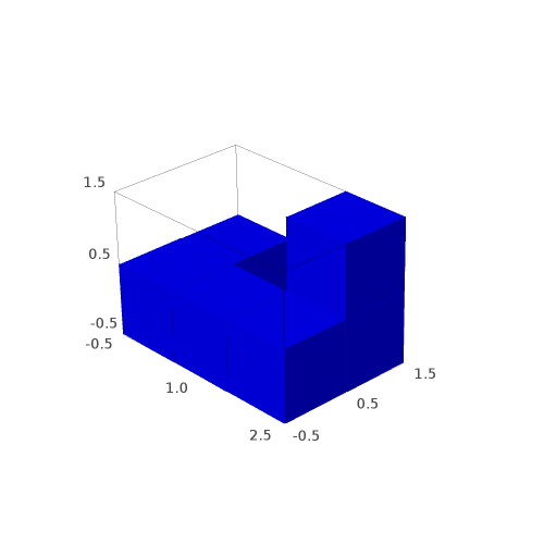
03 décembre 2020 | Catégories: sage, math | View CommentsSuppose that you 3D print many copies of the following 3D hexo-mino at home:
sage: from sage.combinat.tiling import Polyomino, TilingSolver
sage: p = Polyomino([(0,0,0), (0,1,0), (1,0,0), (2,0,0), (2,1,0), (2,1,1)], color='blue')
sage: p.show3d()
Launched html viewer for Graphics3d Object
You would like to know if you can tile a larger polyomino or in particular a rectangular box with many copies of it. The TilingSolver module in SageMath is made for that. See also this recent question on ask.sagemath.org.
sage: T = TilingSolver([p], (7,5,3), rotation=True, reflection=False, reusable=True)
sage: T
Tiling solver of 1 pieces into a box of size 24
Rotation allowed: True
Reflection allowed: False
Reusing pieces allowed: True
There is no solution when tiling a box of shape 7x5x3 with this polyomino:
sage: T.number_of_solutions()
0
But there are 4 solutions when tiling a box of shape 4x3x2 with this polyomino:
sage: T = TilingSolver([p], (4,3,2), rotation=True, reflection=False, reusable=True)
sage: T.number_of_solutions()
4
We construct the list of solutions:
sage: solutions = [sol for sol in T.solve()]
Each solution contains the isometric copies of the polyominoes tiling the box:
sage: solutions[0]
[Polyomino: [(0, 0, 0), (0, 0, 1), (0, 1, 0), (1, 1, 0), (2, 0, 0), (2, 1, 0)], Color: #ff0000,
 Polyomino: [(0, 1, 1), (0, 2, 0), (0, 2, 1), (1, 1, 1), (2, 1, 1), (2, 2, 1)], Color: #ff0000,
 Polyomino: [(1, 0, 0), (1, 0, 1), (2, 0, 1), (3, 0, 0), (3, 0, 1), (3, 1, 0)], Color: #ff0000,
 Polyomino: [(1, 2, 0), (1, 2, 1), (2, 2, 0), (3, 1, 1), (3, 2, 0), (3, 2, 1)], Color: #ff0000]
It may be easier to visualize the solutions, so we define the following function allowing to draw the solutions with different colors for each piece:
sage: def draw_solution(solution, size=0.9):
....:     colors = rainbow(len(solution))
....:     for piece,col in zip(solution, colors):
....:         piece.color(col)
....:     return sum((piece.show3d(size=size) for piece in solution), Graphics())
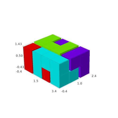
sage: G = [draw_solution(sol) for sol in solutions]
sage: G
[Graphics3d Object, Graphics3d Object, Graphics3d Object, Graphics3d Object]
sage: G[0] # in Sage, this will open a 3d viewer automatically
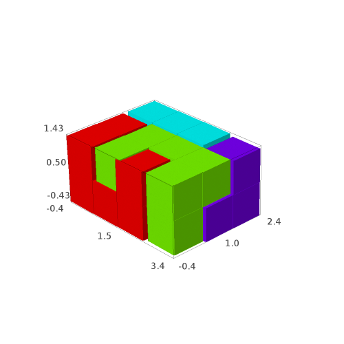
sage: G[1]
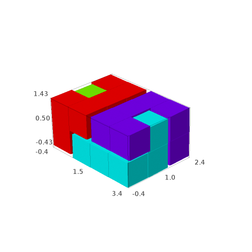
sage: G[2]
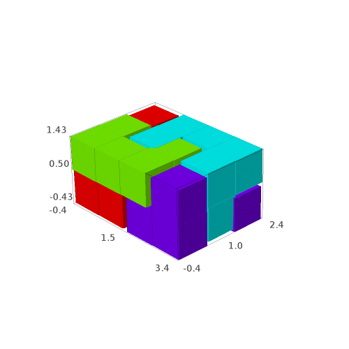
sage: G[3]
We may save the solutions to a file:
sage: G[0].save('solution0.png', aspect_ratio=1, zoom=1.2)
sage: G[1].save('solution1.png', aspect_ratio=1, zoom=1.2)
sage: G[2].save('solution2.png', aspect_ratio=1, zoom=1.2)
sage: G[3].save('solution3.png', aspect_ratio=1, zoom=1.2)
Question: are all of the 4 solutions isometric to each other?
The tiling problem is solved due to a reduction to the exact cover problem for which dancing links Knuth's algorithm provides all the solutions. One can see the rows of the dancing links matrix as follows:
sage: d = T.dlx_solver()
sage: d
Dancing links solver for 24 columns and 56 rows
sage: d.rows()
[[0, 1, 2, 4, 5, 11],
 [6, 7, 8, 10, 11, 17],
 [12, 13, 14, 16, 17, 23],
 ...
 [4, 6, 7, 9, 10, 11],
 [10, 12, 13, 15, 16, 17],
 [16, 18, 19, 21, 22, 23]]
The solutions to the dlx solver can be obtained as follows:
sage: it = d.solutions_iterator()
sage: next(it)
[3, 36, 19, 52]
These are the indices of the rows each corresponding to an isometric copy of the polyomino within the box.
Since SageMath-9.2, the possibility to reduce the problem to a MILP problem or a SAT instance was added to SageMath (see #29338 and #29955):
sage: d.to_milp()
(Boolean Program (no objective, 56 variables, 24 constraints),
 MIPVariable of dimension 1)
sage: d.to_sat_solver()
CryptoMiniSat solver: 56 variables, 2348 clauses.
« Previous Page -- Next Page »
Propulsé par Blogofile
S'abonner au Flux RSS
et aux Commentaires.

This work by Sébastien Labbé is licensed under a Creative Commons Attribution-ShareAlike 4.0 International License.