Tiling a polyomino with polyominoes in SageMath

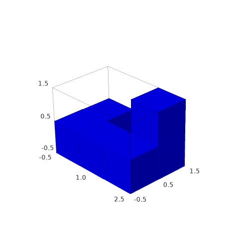
03 décembre 2020 | Catégories: sage, math | View Comments

Suppose that you 3D print many copies of the following 3D hexo-mino at home:

sage: from sage.combinat.tiling import Polyomino, TilingSolver
sage: p = Polyomino([(0,0,0), (0,1,0), (1,0,0), (2,0,0), (2,1,0), (2,1,1)], color='blue')
sage: p.show3d()
Launched html viewer for Graphics3d Object

You would like to know if you can tile a larger polyomino or in particular a rectangular box with many copies of it. The TilingSolver module in SageMath is made for that. See also this recent question on ask.sagemath.org.

sage: T = TilingSolver([p], (7,5,3), rotation=True, reflection=False, reusable=True)
sage: T
Tiling solver of 1 pieces into a box of size 24
Rotation allowed: True
Reflection allowed: False
Reusing pieces allowed: True

There is no solution when tiling a box of shape 7x5x3 with this polyomino:

sage: T.number_of_solutions()
0

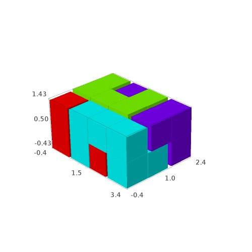
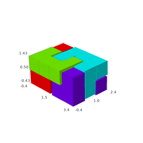
But there are 4 solutions when tiling a box of shape 4x3x2 with this polyomino:

sage: T = TilingSolver([p], (4,3,2), rotation=True, reflection=False, reusable=True)
sage: T.number_of_solutions()
4

We construct the list of solutions:

sage: solutions = [sol for sol in T.solve()]

Each solution contains the isometric copies of the polyominoes tiling the box:

sage: solutions[0]
[Polyomino: [(0, 0, 0), (0, 0, 1), (0, 1, 0), (1, 1, 0), (2, 0, 0), (2, 1, 0)], Color: #ff0000,
 Polyomino: [(0, 1, 1), (0, 2, 0), (0, 2, 1), (1, 1, 1), (2, 1, 1), (2, 2, 1)], Color: #ff0000,
 Polyomino: [(1, 0, 0), (1, 0, 1), (2, 0, 1), (3, 0, 0), (3, 0, 1), (3, 1, 0)], Color: #ff0000,
 Polyomino: [(1, 2, 0), (1, 2, 1), (2, 2, 0), (3, 1, 1), (3, 2, 0), (3, 2, 1)], Color: #ff0000]

It may be easier to visualize the solutions, so we define the following function allowing to draw the solutions with different colors for each piece:

sage: def draw_solution(solution, size=0.9):
....:     colors = rainbow(len(solution))
....:     for piece,col in zip(solution, colors):
....:         piece.color(col)
....:     return sum((piece.show3d(size=size) for piece in solution), Graphics())

sage: G = [draw_solution(sol) for sol in solutions]
sage: G
[Graphics3d Object, Graphics3d Object, Graphics3d Object, Graphics3d Object]

sage: G[0]   # in Sage, this will open a 3d viewer automatically

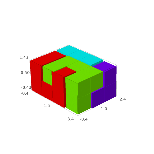
sage: G[1]

sage: G[2]

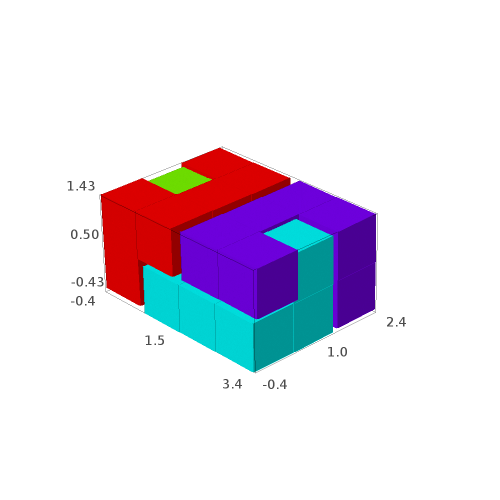
sage: G[3]

We may save the solutions to a file:

sage: G[0].save('solution0.png', aspect_ratio=1, zoom=1.2)
sage: G[1].save('solution1.png', aspect_ratio=1, zoom=1.2)
sage: G[2].save('solution2.png', aspect_ratio=1, zoom=1.2)
sage: G[3].save('solution3.png', aspect_ratio=1, zoom=1.2)

Question: are all of the 4 solutions isometric to each other?

The tiling problem is solved due to a reduction to the exact cover problem for which dancing links Knuth's algorithm provides all the solutions. One can see the rows of the dancing links matrix as follows:

sage: d = T.dlx_solver()
sage: d
Dancing links solver for 24 columns and 56 rows
sage: d.rows()
[[0, 1, 2, 4, 5, 11],
 [6, 7, 8, 10, 11, 17],
 [12, 13, 14, 16, 17, 23],
 ...
 [4, 6, 7, 9, 10, 11],
 [10, 12, 13, 15, 16, 17],
 [16, 18, 19, 21, 22, 23]]

The solutions to the dlx solver can be obtained as follows:

sage: it = d.solutions_iterator()
sage: next(it)
[3, 36, 19, 52]

These are the indices of the rows each corresponding to an isometric copy of the polyomino within the box.

Since SageMath-9.2, the possibility to reduce the problem to a MILP problem or a SAT instance was added to SageMath (see #29338 and #29955):

sage: d.to_milp()
(Boolean Program (no objective, 56 variables, 24 constraints),
 MIPVariable of dimension 1)
sage: d.to_sat_solver()
CryptoMiniSat solver: 56 variables, 2348 clauses.

Sébastien Labbé

Tiling a polyomino with polyominoes in SageMath