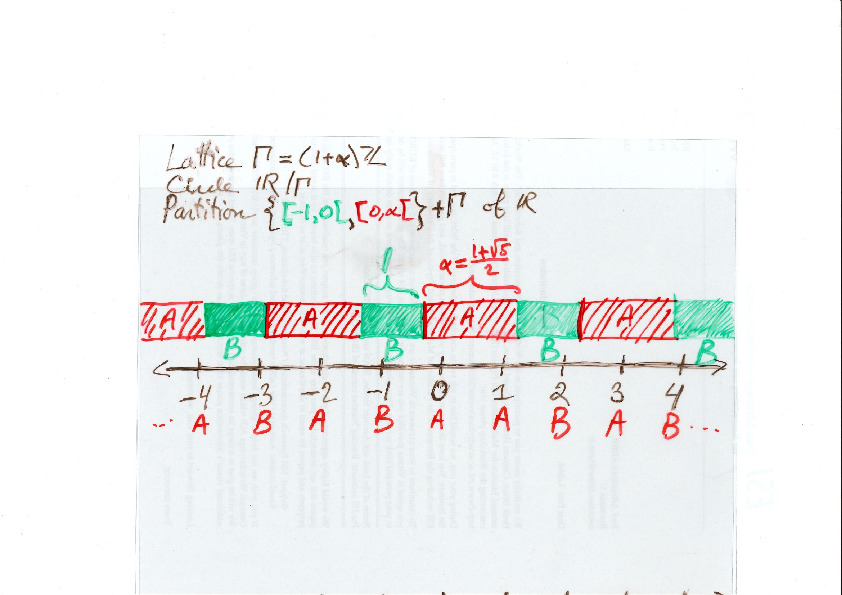
On the bifurcation diagram proposed by Jang and Robinson
06 mai 2025 | Catégories: sage, math | View CommentsIn this blog post, we present a few remarks on the "bifurcation diagram" proposed by Jang and Robinson in [1] to describe the tilings associated to a set of 24 Wang tiles encoding Penrose tilings.
[1] Hyeeun Jang, E. Arthur Robinson Jr, Directional Expansiveness for Rd-Actions and for Penrose Tilings, arxiv:2504.10838
In particular, I believe that something is wrong in what the authors call the "bifurcation diagram" shown in Figure 10. But, as we illustrate below, it can be fixed easily by permuting some of the labels of the partition.
I saw Jang and Robinsion's bifurcation diagram for the first time during the talk "Remembering Shunji Ito" made by Robinson during the online conference dedicated to the memory of Shunji Ito on December 14, 2021. At that time, I was working on the family of metallic mean Wang tiles. This is why the bifurcation diagram shown by Robinson and extracted from Jang's PhD thesis got my attention right away, because it was looking very much like the Markov partition associated to the Ammann set of 16 Wang tiles, the first member of the family of metallic mean Wang tiles. As we illustrate below, Jang and Robinson's bifurcation diagram is a refinement of the Markov partition associated the Ammann set of 16 Wang tiles. This means that the 16 tiles Ammann Wang shift is a factor of the 24 tiles Penrose Wang shift. Also most probably the bifurcation diagram is a Markov Partition for the same associated toral ℤ2-action. But this needs a proof.
The content of this blog post is also available as a Jupyter notebook that can be viewed and downloaded from the nbviewer.
Dependencies
The computations made here depend on the modules WangTileSet, WangTiling, PolyhedronPartition, PolyhedronExchangeTransformation, PETsCoding implemented in the SageMath optional package slabbe over the last years in order to describe and study the Jeandel-Rao aperiodic tilings and the family of metallic mean Wang tiles.
Note that the package slabbe can be installed by running !pip install slabbe directly in SageMath:
sage: # !pip install slabbe # uncomment and execute this line to install slabbe package
Here are the version of the packages used in this post:
sage: import importlib
sage: importlib.metadata.version("slabbe")
'0.8.0'
sage: version()
'SageMath version 10.5.beta6, Release Date: 2024-09-29'
Jang-Robinson encoding of the Penrose 24 Wang tiles
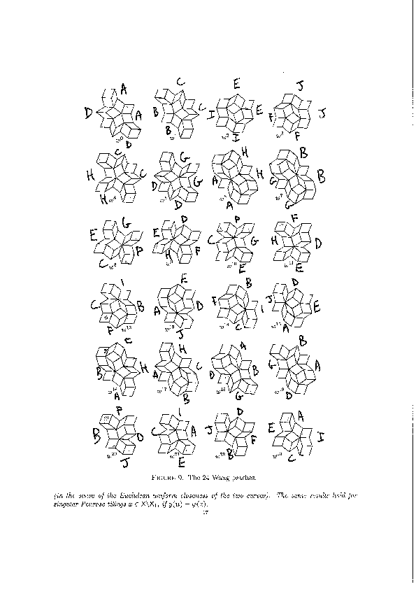
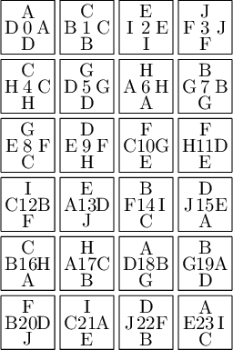
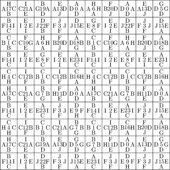
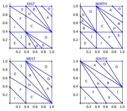
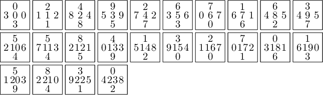
We encode the 24 Wang tiles proposed by Jang and Robinson (Figure 9 of [1]) using alphabet {A, B, C, D, E, F, G, H, I, J} for the shapes:
We define the 24 Wang tiles in SageMath:
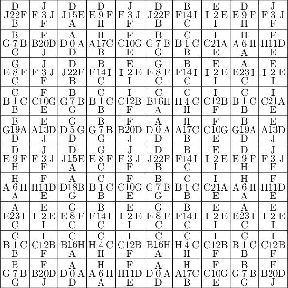
sage: from slabbe import WangTileSet, WangTiling
sage: tiles = ["AADD", "CCBB", "EEII", "JJFF",
....:          "CCHH", "GGDD", "HHAA", "BBGG",
....:          "FGEC", "FDEH", "GFCE", "DFHE",
....:          "BICF", "DEAJ", "IBFC", "EDJA",
....:          "HCBA", "CHAB", "BADG", "ABGD",
....:          "DFBJ", "AICE", "FDJB", "IAEC"]
sage: T0 = WangTileSet([tuple(str(a) for a in tile) for tile in tiles])
sage: T0
Wang tile set of cardinality 24
sage: T0.tikz(ncolumns=4)
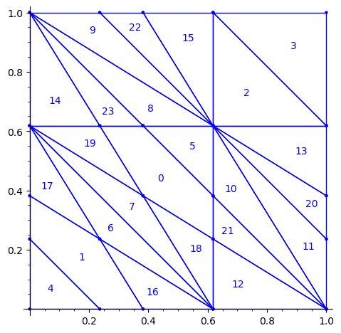
Constructing Jang-Robinson Bifurcation diagram as a polygonal partition
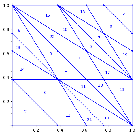
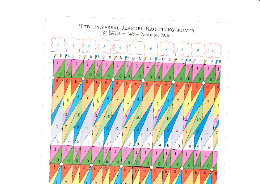
Below is a reproduction of Jang-Robinson bifurcation diagram shown in Figure 10 from arxiv:2504.10838
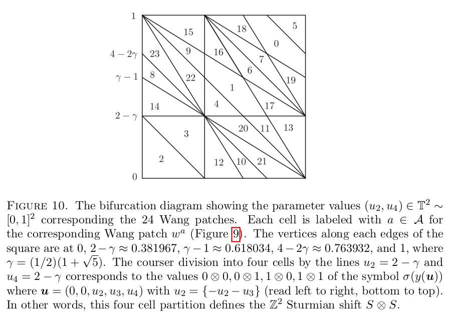
In this section, we construct this bifurcation diagram in SageMath as a polygonal partition.
sage: from slabbe import PolyhedronPartition
sage: z = polygen(QQ, 'z')
sage: K = NumberField(z**2-z-1, 'phi', embedding=RR(1.6))
sage: phi = K.gen()
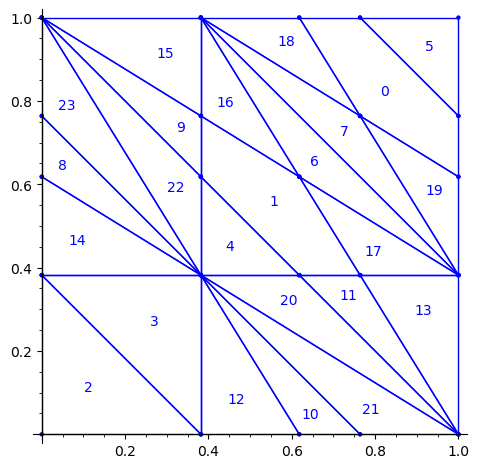
sage: square = polytopes.hypercube(2,intervals = 'zero_one')
sage: P = PolyhedronPartition([square])
sage: P = P.refine_by_hyperplane([1/phi^3,-1,-1])
sage: P = P.refine_by_hyperplane([1/phi,-1,-1])
sage: P = P.refine_by_hyperplane([1,-1,-1])
sage: P = P.refine_by_hyperplane([1 + 1/phi,-1,-1])
sage: P = P.refine_by_hyperplane([1 + 1/phi^3,-1,-1])
sage: P = P.refine_by_hyperplane([1/phi,-phi,-1])
sage: P = P.refine_by_hyperplane([1,-phi,-1])
sage: P = P.refine_by_hyperplane([phi,-phi,-1])
sage: P = P.refine_by_hyperplane([1/phi^2,-1/phi,-1])
sage: P = P.refine_by_hyperplane([1/phi,-1/phi,-1])
sage: P = P.refine_by_hyperplane([1,-1/phi,-1])
sage: P = P.refine_by_hyperplane([1/phi,-1,0])
sage: P = P.refine_by_hyperplane([1/phi,0,-1])
sage: P = -P
sage: P = P.translate((1,1))
sage: #P.plot()
sage: P = P.rename_keys({0:5, 1:0, 2:18, 3:19, 4:7, 5:6, 6:16, 7:17, 8:1, 9:4, 10:15,11:9,
sage:                    12:22,13:23,14:8, 15:14,16:13,17:11,18:20,19:21,20:10, 21:12, 22:3,
sage:                    23:2})
sage: P.plot()
Our claim
We claim that the above bifurcation diagram from Jang-Robinson preprint is slightly wrong according to the choice of indices of the 24 Wang tiles made by Jang and Robinson and shown above. The following changes should be made in order to fix the partition:
- indices 9 and 22 should be swapped,
- indices 8 and 23 should be swapped,
- indices 11 and 20 should be swapped and
- indices 10 and 21 should be swapped.
Defining the toral translations in the internal space as PETs
We define the toral translations associated to the partition chosen by Jang-Robinson. The internal space is the 2-dimensional torus ℝ2 ⁄ ℤ2. It is represented as the unit square [0, 1)2. On this fundamental domain, a toral translation is a polygon exchange transformation.
Note that according to their choice,
- a unit horizontal translation in the physical space corresponds to a vertical translation by (0, φ) in the internal space,
- a unit vertical translation in the physical space corresponds to a horizontal translation by (φ, 0) in the internal space,
where φ is the golden mean.
Below, we follow their convention.
sage: from slabbe import PolyhedronExchangeTransformation as PET
sage: base = diagonal_matrix((1,1))
sage: R0e1 = PET.toral_translation(base, vector((0,phi)))
sage: R0e2 = PET.toral_translation(base, vector((phi,0)))
We compute a 10×10 pattern obtained by coding the orbit of some starting point under the ℤ2-action R0.
sage: from slabbe.coding_of_PETs import PETsCoding
sage: coding_R0_P = PETsCoding((R0e1,R0e2), P)
sage: pattern = coding_R0_P.pattern((.3,.4), (10,10))
sage: pattern = WangTiling(pattern, T0)
sage: pattern.tikz()
We observe that this pattern is not valid !!!
Let's fix the partition
We claim that the above pattern is wrong because something is wrong in the labelling of the atoms in the partition proposed by Jang and Robinson for the 24 Wang tiles encoding Penrose tilings.
Below, we fix the partition by swapping labels 8 and 23, 9 and 22, 11 and 20, 10 and 21:
sage: d = {i:i for i in range(24)}
sage: d.update({8:23, 23:8, 9:22, 22:9, 11:20, 20:11, 10:21, 21:10})
sage: P1 = P.rename_keys(d)
sage: P1.plot()
We compute a 10×10 pattern out of this updated partition P1:
sage: coding_R0_P1 = PETsCoding((R0e1,R0e2), P1)
sage: pattern = coding_R0_P1.pattern((.3,.4), (10,10))
sage: pattern = WangTiling(pattern, T0)
sage: pattern.tikz()
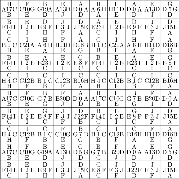
We observe that this pattern is valid !!!
Understanding the issue using edge label partitions
Let us try to understand the fix in terms of the Wang tiles east, north, west and south edge labels partitions induced by the original partition.
Indeed, since each atom of the partition corresponds to a Wang tile, we can deduce a partition of the unit square for the east labels (and respectively for the north, west and south labels) by merging two atoms in the partition if their east edge label is the same.
sage: def edge_label_partitions(partition, tiles):
....:     EAST = partition.merge_atoms({i:tiles[i][0] for i in range(24)})
....:     NORTH = partition.merge_atoms({i:tiles[i][1] for i in range(24)})
....:     WEST = partition.merge_atoms({i:tiles[i][2] for i in range(24)})
....:     SOUTH = partition.merge_atoms({i:tiles[i][3] for i in range(24)})
....:     return EAST, NORTH, WEST, SOUTH
sage: def draw_edge_label_partitions(partition, tiles):
....:     EAST, NORTH, WEST, SOUTH = edge_label_partitions(partition, tiles)
....:     L = [EAST.plot() + text('EAST', (.5,1.05)),
....:          NORTH.plot() + text('NORTH', (.5,1.05)),
....:          WEST.plot() + text('WEST', (.5,1.05)),
....:          SOUTH.plot() + text('SOUTH', (.5,1.05))]
....:     return graphics_array(L, nrows=2)
This is what we get using the partition proposed by Jang and Robinson for the 24 Wang tiles encoding Penrose tilings:
sage: draw_edge_label_partitions(P, T0)
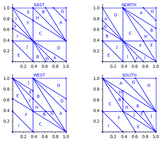
Here are some observations which are normal:
- partitions NORTH and EAST are symmetric under a reflexion by the positive diagonal (remember that the tile set is symmetric under the positive diagonal)
- partitions WEST and SOUTH are symmetric under a reflexion by the positive diagonal (remember that the tile set is symmetric under the positive diagonal)
Here are some observations which are not normal:
- partitions WEST and EAST do not give the same area to the same index (in a Wang tiling, the frequency of a EAST label should be equal to the frequency of the same WEST label)
- partitions SOUTH and NORTH do not give the same area to the same index (in a Wang tiling, the frequency of a NORTH label should be equal to the frequency of the same SOUTH label)
- partitions EAST and WEST are not a translate of one another (idealy a horizontal translate)
- partitions SOUTH and NORTH are not a translate of one another (idealy a vertical translate)
Another indication that something may be wrong is:
- atoms B, H, E, J, A, G are not convex in the torus
This is not a necessity. Atoms are not convex in the Markov partition associated to Jeandel-Rao tilings [2]. But they are convex for the Ammann set of 16 Wang tiles and their generalization to metallic mean numbers made in [3,4]. Since Penrose tilings are closely related to Ammann A2 tilings, we may also expect to have simple convex atoms in each of the four edge label partitions.
Here is the area of each atom in each of the four partitions. We observe that only atoms C and D have the same area in each of the four partitions.
sage: def table_of_area_of_atom_in_east_north_west_south_partitions(partition, tiles):
....:     columns = []
....:     labels = 'ABCDEFGHIJ'
....:     EAST, NORTH, WEST, SOUTH = edge_label_partitions(partition, tiles)
....:     for partition in [EAST, NORTH, WEST, SOUTH]:
....:         d = partition.volume_dict()
....:         column = [d[a] for a in labels]
....:         columns.append(column)
....:     header_row = ['EAST', 'NORTH', 'WEST', 'SOUTH']
....:     return table(columns=columns, header_row=header_row, header_column=['']+list(labels))
sage: table_of_area_of_atom_in_east_north_west_south_partitions(P, T0)
    │ EAST             NORTH            WEST             SOUTH
├───┼────────────────┼────────────────┼────────────────┼────────────────┤
  A │ 15/2*phi - 12    15/2*phi - 12    phi - 3/2        phi - 3/2
  B │ phi - 3/2        phi - 3/2        15/2*phi - 12    15/2*phi - 12
  C │ phi - 3/2        phi - 3/2        phi - 3/2        phi - 3/2
  D │ phi - 3/2        phi - 3/2        phi - 3/2        phi - 3/2
  E │ phi - 3/2        phi - 3/2        -11/2*phi + 9    -11/2*phi + 9
  F │ -11/2*phi + 9    -11/2*phi + 9    phi - 3/2        phi - 3/2
  G │ -8*phi + 13      -8*phi + 13      -3/2*phi + 5/2   -3/2*phi + 5/2
  H │ -3/2*phi + 5/2   -3/2*phi + 5/2   -8*phi + 13      -8*phi + 13
  I │ 5*phi - 8        5*phi - 8        -3/2*phi + 5/2   -3/2*phi + 5/2
  J │ -3/2*phi + 5/2   -3/2*phi + 5/2   5*phi - 8        5*phi - 8
But, we observe that we can fix the partitions if we assume that the atoms C and D in the four partitions are correct. There is a unique translation sending atoms C,D in the partition WEST to the atoms C and D in the partition EAST. That translation should send the partition WEST exactly on EAST. Similarly for SOUTH and NORTH. This suggest a way to fix atoms B, H, E, J, A, G in the partition.
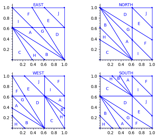
Fixed Edge labels partitions
Using the fixed partition, here is what we get.
sage: P1.plot()

sage: draw_edge_label_partitions(P1, T0)
Now it looks good! As for the partitions associated to the metallic mean Wang tiles, the four partitions are isometric copies of the other ones (under toral translation or reflection).
sage: table_of_area_of_atom_in_east_north_west_south_partitions(P1, T0)
    │ EAST             NORTH            WEST             SOUTH
├───┼────────────────┼────────────────┼────────────────┼────────────────┤
  A │ phi - 3/2        phi - 3/2        phi - 3/2        phi - 3/2
  B │ phi - 3/2        phi - 3/2        phi - 3/2        phi - 3/2
  C │ phi - 3/2        phi - 3/2        phi - 3/2        phi - 3/2
  D │ phi - 3/2        phi - 3/2        phi - 3/2        phi - 3/2
  E │ phi - 3/2        phi - 3/2        phi - 3/2        phi - 3/2
  F │ phi - 3/2        phi - 3/2        phi - 3/2        phi - 3/2
  G │ -3/2*phi + 5/2   -3/2*phi + 5/2   -3/2*phi + 5/2   -3/2*phi + 5/2
  H │ -3/2*phi + 5/2   -3/2*phi + 5/2   -3/2*phi + 5/2   -3/2*phi + 5/2
  I │ -3/2*phi + 5/2   -3/2*phi + 5/2   -3/2*phi + 5/2   -3/2*phi + 5/2
  J │ -3/2*phi + 5/2   -3/2*phi + 5/2   -3/2*phi + 5/2   -3/2*phi + 5/2
sage: (phi-3/2).n(), (-3/2*phi + 5/2).n()
(0.118033988749895, 0.0729490168751576)
Labels A, B, C, D, E and F all have the same frequency of ϕ − (3)/(2) ≈ 0.118.
Labels G, H, I and J all have the same frequency of − (3)/(2)ϕ + (5)/(2) ≈ 0.0729.
We check that frequencies sum to 1:
sage: 6 * (phi-3/2) + 4 * (-3/2*phi + 5/2)
1
Proposed partition for the encoding of the Penrose tilings into 24 Wang tiles
As done with the Markov partition associated to Jeandel-Rao aperiodic tilings, and for the Markov partition associated to the family of metallic mean Wang tiles, I think it is more natural to associate horizontal (vertical) translations in the internal space with horizontal (vertical) translations in the physical space. This way, the brain is less mixed up and the projections in the physical space π and in the internal space πint of the cut and project scheme are defined more naturally. This way the internal space and physical space can even be identified: this is the root of the do-it-yourself tutorial allowing the construction of Jeandel-Rao tilings [5]. See also my Habilitation à diriger des recherches written in English during Spring 2025 for more information [6].
First, we flip the partition P1 by the positive diagonal. This exchanges the role of x and y axis.
sage: P2 = P1.apply_linear_map(matrix(2, [0,1,1,0]))
sage: P2.plot()

This allows to define the ℤ2-action R1 on the torus with horizontal and vertical translations for e1 and e2 respectively:
sage: base = diagonal_matrix((1,1))
sage: R1e1 = PET.toral_translation(base, vector((1/phi,0)))
sage: R1e2 = PET.toral_translation(base, vector((0,1/phi)))
Then, we rotate the partition. This changes the origin of the partition. This change may be optional, but it makes the partition look closer to the partitions already studied in [2,3,4]. It simplifies the explanation of any relation between them (and there is one, see below!).
sage: P3 = R1e1(P2)
sage: P3 = R1e2(P3)
sage: P3.plot()
We observe that the partition P3 associated to the 24 Wang tiles encoding Penrose tiling is a refinement of the partition associated to the 16 Ammann tiles (see Figure 15 in [4] as the 16 Ammann tiles are equivalent to the n-th metallic mean Wang tiles when n = 1).
We compute a 10×10 pattern obtained by coding the orbit of some starting point under the ℤ2-action R1 using partition P3.
sage: from slabbe.coding_of_PETs import PETsCoding
sage: coding_R1_P3 = PETsCoding((R1e1,R1e2), P3)
sage: pattern = coding_R1_P3.pattern((.3,.4), (10,10))
sage: pattern = WangTiling(pattern, T0)
sage: pattern.tikz()
We are happy to see that the pattern is still valid after all the changes we have made!
sage: draw_edge_label_partitions(P3, T0)
We observe that the EAST, NORTH, WEST and SOUTH partitions are a refinement of the EAST, NORTH, WEST and SOUTH partitions associated to the Ammann tiles partition (see Figure 15 in [4]).
The difference between the Ammann EAST and 24 Wang tiles Penrose EAST partition is the addition of two closed geodesics of slope -1 on the 2-torus passing through the origin and through the vertex (0, φ − 1).
It is possible that there is a clever way of including this information into the labels of the Wang tiles as we have done it for the family of metallic mean Wang tiles. Possibly, we need to use 4-dimension vectors for the tile labels instead of 3-dimensional integer vectors. This remains an open question.
Wang tiles deduced from the partition and ℤ2-action
We check that the Wang tiles computed from the partition P3 and ℤ2-action R1 is the original set of 24 Wang tiles defined by Jang and Robinson.
See Proposition 8.1 in [2].
sage: T = coding_R1_P3.to_wang_tiles()
sage: T.tikz()
sage: T.is_equivalent(T0, certificate=True)
(True,
 {'3': 'D',
  '0': 'A',
  '6': 'G',
  '1': 'B',
  '7': 'H',
  '2': 'C',
  '8': 'I',
  '4': 'E',
  '5': 'F',
  '9': 'J'},
 {'3': 'D',
  '0': 'A',
  '6': 'G',
  '1': 'B',
  '7': 'H',
  '2': 'C',
  '8': 'I',
  '4': 'E',
  '5': 'F',
  '9': 'J'},
 Substitution 2d: {0: [[0]], 1: [[1]], 2: [[2]], 3: [[3]], 4: [[4]], 5:
 [[5]], 6: [[6]], 7: [[7]], 8: [[8]], 9: [[9]], 10: [[10]], 11: [[11]], 12:
 [[12]], 13: [[13]], 14: [[14]], 15: [[15]], 16: [[16]], 17: [[17]], 18: [[18]],
 19: [[19]], 20: [[20]], 21: [[21]], 22: [[22]], 23: [[23]]})
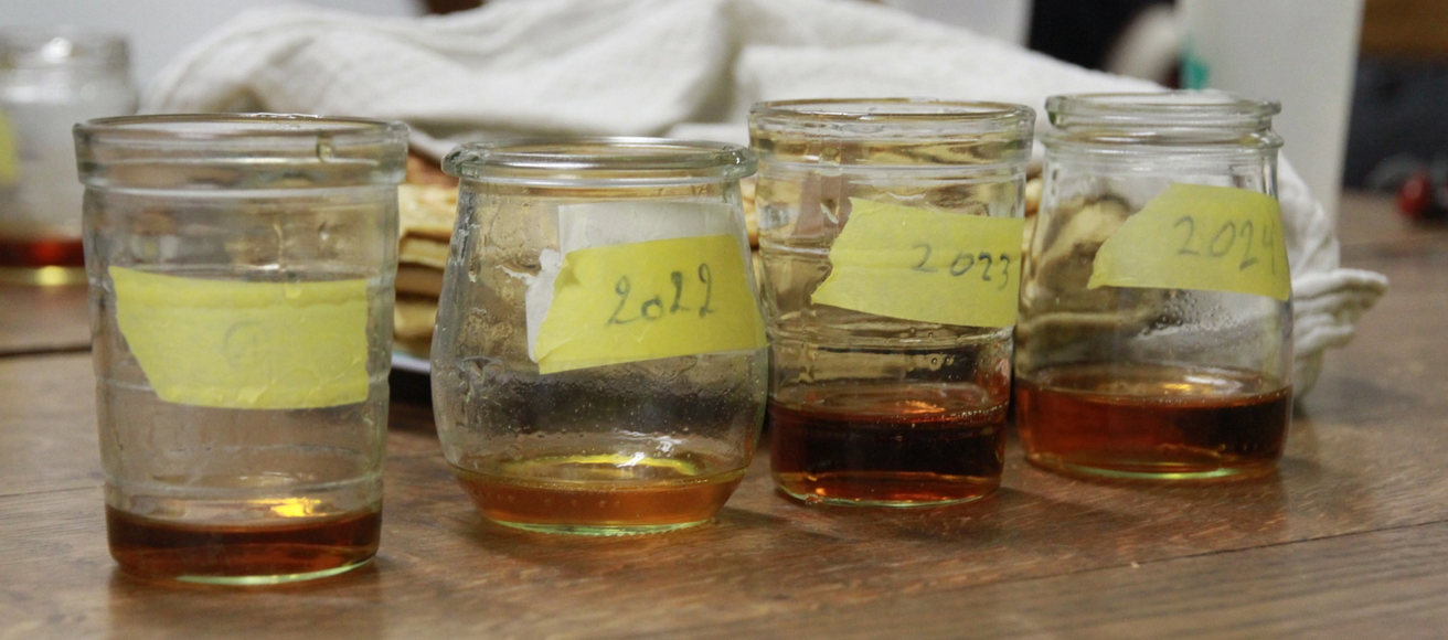
Dégustation de sirop d'érable à Bègles
12 mars 2025 | Catégories: Uncategorized | View CommentsLe 12 mars 2025, nous avons organisé une dégustation de sirop d'érable à Bègles, à la zone à partager, avec l'aide de notre ami Jérémy qui organise régulièrement des dégustations de vin. L'objectif étant de partager ce qu'est le temps des sucres en profitant de l'expérience bordelaise dans la dégustation de vin. Pour ce faire, on se base sur les travaux récents d'Agriculture Canada qui propose une roue des flaveurs pour repérer les saveurs des produits de l'érable.
En 2022, nous avions organisé une dégustation au même endroit où on avait dégusté des sirops de différentes régions du Québec. La dégustation du 12 mars 2025 avait la particularité d'être une dégustation verticale, c'est-à-dire, comme dans le vin, on goûte des millésimes consécutifs du sirop provenant de la même cabane à sucre. Plus précisément, nous avons goûté au sirop de 2022, 2023 et 2024 de la cabane à sucre de ma tante Diane et mon oncle Guy Roy de Sainte-Cécile-de-Whitton près de Lac-Mégantic.
Quelques jours avant la dégustation, Guy m'a rappelé les particularité de chacune des saisons hivernales. En voici un résumé:
- 2008: mauvaise saison, il tombe 2 pieds de neige le 23 mars (anniversaire André Roy), le rang 9 est bouché pendant 2 jours, trop neige au printemps, les températures au sol restent froides : 32 barils
- 2019: la saison termine tard (début mai)
- 2020: la saison termine tard (début mai)
- 2022: ça coule du 17 mars au 27 avril : 132 barils (plus de neige, très bonne saison quand même)
- 2023: ça coule du 24 mars au 16 avril : 55 barils (la saison se termine avec -20 degrés et beaucoup de neige, ensuite ça ne coulait pas, moitié du quota)
- 2024: ça coule du 28 février au 17 avril : 126 barils (peu de neige, mais bonne saison)
Voici les dégustations du 12 mars 2025:
- Le sirop du Leclerc, magasin supermarché en France
- Le sirop de Diane et Guy Roy, rang 9, Sainte-Cécile (Estrie)
- 2022, "plus de neige, volume record, 132 barils"
- 2023, "trop de neige tardivement, 55 barils"
- 2024, "peu de neige, 126 barils"
- Le sirop de Tem-Sucre (Témiscamingue)
C'est toujours intéressant de commencer la dégustation avec un sirop de la grande distribution. Cette année on a commencé avec celui du magasin Leclerc. En 2022, on avait commencé avec celui du Spar.
J'ai été surpris de constater que les trois saisons 2022, 2023, 2024 du sirop familial n'ont pas la même odeur, ni la même couleur, ni le même goût. En particulier, j'ai trouvé que la saison 2023 avait le plus de saveur. Le goût de l'érable du sirop de 2023 était plus développé que les deux autres années. Peut-être que la plus petite quantité produite dans la saison donne plus de temps pour bouillir le sirop tranquillement? Je dois en parler avec mon oncle et ma tante pour vérifier cette hypothèse!
Voici le vidéo que nous avons regardé le 12 mars 2025 avant la dégustation:
Voici d'autres vidéos qui montrent bien le temps des sucres au Québec:
- La semaine verte : Histoires de sève - 8 mars 2022
- La semaine verte : Flaveurs du sirop d’érable - 1 mars 2021
- La semaine verte : Coulée hâtive des érables - 23 avril 2024
- Radio-Canada : préserver les méthodes d’antan - 15 avril 2022
- Est-ce qu’un Québécois peut faire du sirop d’érable sans expérience ?
Un vidéo de passe-partout de 1979 pour les enfants :
Des idées pour le mandat 2025-2028 de la FFFD
23 janvier 2025 | Catégories: ultimate | View CommentsJ'ai suivi la campagne électorale de la Fédération française de Flying Disc de l'automne 2024 avec intérêt, vue la présence de deux listes, mais de loin, car j'étais en déplacement en novembre 2024. J'ai trouvé le débat entre les deux listes du 11 novembre 2024 rafraîchissant et inspirant (merci beaucoup à Focus Ultimate pour l'avoir organisé). Peu importe qui remporte les élections, le fait de discuter et débattre de l'organisation de l'ultimate en France est nécessaire et doit être fait de façon régulière pour prendre du recul, comprendre les problèmes vécus par les clubs et améliorer les choses. Suite à ce débat, j'avais pris plusieurs idées en note. Je viens enfin de prendre le temps de les mettre sur papier.
J'aimerais donc profiter de cette élection qui vient de se dérouler pour partager à la nouvelle équipe en place quelques réflexions au sujet de l'organisation de l'ultimate en France. Elles sont déclinées ci-bas section par section.
Anticiper la croissance
À mon avis, la première règle qui doit guider la nouvelle équipe en place à la FFFD est d'anticiper la croissance et de prendre les décisions sur tous les sujets en conséquence. Selon le rapport annuel de la FFFD, il y avait 6648 adhérents pour l'année 2023-2024. Soyons honnête, ce nombre d'adhérents à un sport est très très bas pour un pays comme la France. Les plus récents chiffres de l'INSEE parlent de 2 millions d'adhérents au football, 1 millions d'adhérents au tennis, 675 000 pour l'équitation, 594 000 pour le basketball, 531 000 pour le handball, 529 000 pour le judo, 374 000 pour le rugby, 68 000 pour les échecs, 60 000 pour le kick-boxing, muay-thaï et disciplines associées. Le Flying Disc ne fait pas partie du tableau.
Toutefois, cela démontre tout le potentiel de développement de l'ultimate en France au cours des prochaines années. À mon avis, il est honnête de viser comme objectif d'avoir 50 000 adhérents d'ici quelques années. Or, pour y arriver, il faut construire dès aujourd'hui les structures fédérales comme si on avait déjà 50 000 adhérents.
Par exemple, veut-on avoir un employé à la fédération qui regarde tous les pdf des certificats médicaux de tous les adhérents à la fédération? On peut donner cette tâche à un employé pour quelques centaines d'adhérents, mais on ne veut et on ne peut certainement pas le faire lorsqu'on a 50 000 documents à vérifier.
Ceci n'est qu'un exemple, mais il y en a plusieurs autres. De façon générale, n'attendons pas d'avoir 50 000 adhérents pour être capable de les gérer. Prenons les décisions dès maintenant comme si on avait déjà 50 000 adhérents.
Tout doit être réfléchis et mis en place pour que doubler le nombre d'ahérents en France ne fasse pas doubler le travail des employés et bénévoles fédéraux.
Think big sti
Think big comme dit Elvis Gratton (joué par le comédien Julien Poulin, que les Québécois aiment tous beaucoup, et qui est décédé le 4 janvier 2025): visons d'avoir 50 000 adhérents à la fédération d'ici 10 ans, pas 25 ans. Rappelons que cela a pris 25 ans à la FFFD pour multiplier par dix le nombre d'adhérents en passant de quelques centaines à quelques milliers.
Cela représente une croissance de 25% par année, plutôt que l'actuel 10%. Pour y arriver, il va falloir changer de paradigme. Les clubs devront s'y mettre : accueillir les nouveaux et nouvelles joueuses d'une façon à les fidéliser peu importe leur niveau de jeu. Le rôle de la fédération est de mettre les structures en place pour y arriver. Comment récompenser les clubs qui connaissent une augmentation de 25 %?
Une croissance de 25% par année, cela signifie doubler le nombre d'adhérents à chaque 3 ans. Cela veut aussi dire doubler le budget des cotisations à la fédération à chaque trois ans.
Ici, on peut rappeler que la cotisation des membres joueurs à la fédération a été augmentée de 1 EUR par année pendant quelques années avant et après la pandémie pour rejoindre 57 EUR pour la licence adulte compétition. C'est donc maintenant plus élevé que la cotisation à la fédération française de judo. Sous l'hypothèse d'une stagnation du nombre de licenciers, cela permet d'augmenter le budget de la fédération provenant des cotisations de 2% par année. J'avais trouvé cette décision plutôt triste, car je l'interprétais comme une abdication face à la responsabilité d'augmenter le nombre de pratiquants en France. En effet, si on prend conscience du potentiel de développement de la pratique de l'ultimate, on comprend que l'augmentation du budget de la fédération proviendra d'abord et avant tout de la croissance du nombre de licenciés. Doubler le nombre de licenciés signifie doubler la part du budget de la fédération provenant des cotisations.
Pour y arriver, il ne suffira pas de récompenser les clubs qui connaissent une croissance. Il va falloir que pratiquer l'ultimate devienne une passion hyper-contagieuse. Ici, je ne veux pas dire de faire des soirées dans tous les sens. Oui, bien sûr, c'est très bien, mais ce n'est pas ce qui est le plus nécessaire.
Développer la passion chez les adhérents est beaucoup plus subtil.
Développer la passion: permettre aux clubs de réaliser leur potentiel
Ici, je trouve plus simple d'expliquer la passion par son contraire. Fermer les yeux et réfléchissez à vos dernières années de compétition en ultimate. Avez-vous déjà vécu des frustrations à la fin d'une saison, non pas à cause de vos défaites, mais à cause de l'organisation de l'ultimate? Si oui, alors ces frustrations empêchent le développement de la passion.
Peut-être les horaires des championnats? des injustices? des joueurs qui quittent vos équipes pour aller jouer dans une équipe de D1 plutôt qu'avec vous? les matchs de la phase 1 d'un championnat annulée à cause de l'annulation de la phase 2 pour certaines équipes à cause de la pluie? remporter tous les matchs en régional et terminer sans aucune défaite ni même d'opposition intéressante? viser la première place en D3 et terminer deuxième en ayant gagner contre l'équipe qui monte en D2 suite à une triple égalité en tête (+1,+0,-1) après un round robin à 13 équipes? Ce sont plein d'histoires que j'ai entendues ces dernières années, mais vous en avez probablement d'autres en tête. Chacune de ces histoires sont loin d'être passionnantes et donnent plutôt envie de pleurer ou de changer de sport.
La passion, c'est l'état mental d'un joueur/euse ou d'un club qui donne envie de revivre la même expérience et faire mieux, qui donne envie d'inviter d'autres personnes à se joindre à nous pour vivre ce qu'on vit et qui, in fine, favorise la croissance.
La fédération permet à la passion de se développer lorsque le système en place récompense avec très haute probabilité les grands efforts nécessaires pour devenir champion.
Mon opinion est que la passion au niveau d'un club se développe lorsqu'on permet aux clubs de réaliser leur plein potentiel dans un temps raisonnable (deux à trois ans). La réalisation du potentiel d'un club étant mesurée annuellement lors les compétitions fédérales, d'où l'importance de leur bon fonctionnement.
Aussi, pour reprendre la terminologie de la pyramide de Maslow, les clubs ont besoin de "reconnaissance et d'appréciation des autres". Idéalement, les classements des championnats de France, s'ils sont bien structurés, doivent donner une représentation la plus fidèle possible de la force relative des clubs et des équipes pour permettre cette reconnaissance. Plus les classements extraits des Championnats de France seront fidèles à la réalité, plus les clubs se passionneront pour y être bien classés, car synonymes de reconnaissance.
Développer la croissance et la passion: Objectifs contradictoires?
Mais alors, comment joindre ces deux objectifs qui semblent à prime abord plutôt contradictoires?
Déjà, si on multiplie par 10 le nombre d'équipes dans les Championnats de France national + régional, alors il faudra aussi multiplier par 10 le nombre de divisions au niveau national et/ou au niveau régional. Or, ça va prendre une éternité à un nouveau club d'athlètes avec un grand potentiel pour atteindre son plein potentiel avec le système actuel.
Pensez-vous sérieusement que 15 athlètes de 19 ans vont attendre patiemment les montées successives de divisions régionales puis nationales au rythme d'une montée par année si on est optimiste? Non, au mieux, ils vont tenter d'être recrutés dans des clubs déjà en N1. Au pire, ils vont changer de sport.
En conservant le fonctionnement actuel et en multipliant par 10 le nombre de pratiquants d'ultimate en France, il n'y a aucune chance qu'une équipe réalise son plein potentiel avec une multiplication par 10 des niveaux et catégories.
En pratique (et malheureusement), ce problème devient la solution. En effet, si ça devient si pénible de jouer à l'ultimate sous l'hypothèse d'une forte augmentation du nombre d'adhérents, alors le nombre d'adhérents cessera d'augmenter. C'est la loi de l'offre et la demande. On peut même se demander si cette loi a déjà fait effet? On peut certainement penser que oui, car le même système actuel est utilisé depuis des années et des années. Le système actuel a donc certainement atteint un point d'équilibre.
Il est important de réfléchir à comment préserver la passion des clubs (surtout les nouveaux clubs avec forts potentiels dans les divisions de bas niveau, régional, etc.) sous l'hypothèse d'une multiplication forte du nombre d'adhérents.
À mon avis, si on veut éviter la contradiction entre favoriser la croissance et la passion, il faut repenser le système des compétitions d'ultimate en France.
Particularité de l'ultimate France: l'embarras du choix
"La vie est un choix. Faire un choix est un choix, ne pas en faire en est un aussi." - Citation sur la vie.
"Nous sommes nos choix" Jean-Paul Sartre.
Ce qui est merveilleux avec l'ultimate en France est qu'on peut pratiquer l'ultimate sur les trois surfaces:
- il y a des plages magnifiques sur l'océan Atlantique et la mer Méditerranée,
- il existe des gymnases handball de qualité,
- il existe des terrains de football et de rugby.
Pratiquer l'ultimate sur les trois surfaces est une chance, car cela n'est pas le cas de tous les pays. Plusieurs pays n'ont pas d'accès à l'océan et n'ont pas de plage comme en France. Dans les pays nordiques, la neige recouvre les terrains extérieurs une bonne partie de l'année, etc.
Cela divise naturellement la saison de compétitions en trois quadrimestres (beach de juillet à octobre, indoor de novembre à février et outdoor de mars à juin).
En plus d'avoir des saisons de compétitions raccourcies par la présence des trois surfaces, l'organisation de l'ultimate en France se démarque d'une autre façon. Pour les trois surfaces, on peut participer à la fois aux compétitions en catégorie mixte et open (ou mixte et féminin pour les femmes).
Dans certains pays, l'organisation de l'ultimate fait en sorte qu'on ne peut pas participer dans la catégorie mixte et open dans la même saison, simplement parce que le championnat mixte, féminin et open a lieu en même temps. C'est souvent d'ailleurs le cas pour les compétitions internationales.
Comme plusieurs personnes, j'adore jouer en mixte et en open. Et comme on ne veut pas choisir, on désire avoir la possibilité de s'inscrire dans les deux catégories dans la même saison. Ici, mon objectif est simplement de faire prendre conscience que cette situation n'est pas une fatalité, mais bien un choix. Un choix de la fédération. C'est un choix qu'on peut continuer de faire. C'est aussi un choix qu'on peut changer. Dans tous les cas, ce choix a des avantages ET des inconvénients et il est important de se poser la question de façon régulière si les avantages restent supérieurs aux inconvénients.
Dans certains pays, on forme et prépare une équipe d'ultimate mixte, open ou féminine pendant les 8 mois avant la compétition majeure annuelle. En France, cette durée est souvent réduite à 2 mois d'entraînement avec tous les joueurs exclusivement concentrés sur la compétition visée. Cela n'est pas une fatalité, mais bien un choix très important fait par la fédération.
Parmi les inconvénients du statu quo, on peut lister les suivants:
- le calendrier, déjà comprimé en quadrimestres par les trois saisons/surfaces, doit en plus éviter les chevauchements des compétitions entre les catégorie mixte, féminines et masculines.
- les clubs doivent optimiser leur performance quasi parallèlement pour des compétitions mixtes et open/féminines. La préparation physique d'un athlète et d'une équipe pour atteindre des peak n'est pas mon expertise de recherche. Mais selon mon expérience personnelle, je trouve qu'encadrer la préparation d'une équipe mixte et open en parallèle est sous-optimale.
Parmi les avantages à orienter les joueurs à faire un choix entre une participation dans une équipe mixte ou open/féminin, il y a:
- assouplissement des contraintes imposées au calendrier fédéral;
- orienter les clubs, les équipes et les joueurs à faire des choix et s'investir pleinement dans ceux-ci pour atteindre une qualité de jeu en équipe jamais vue auparavant;
- ne pas laisser les quelques meilleurs joueurs d'un club saturer toutes les opportunités de jeu.
- augmenter le nombre total de joueurs/euses: pour participer à deux ou trois catégories (mixte et open, mixte et féminin ou les trois), les clubs seront à la recherche de joueurs et de joueuses pour remplir leurs équipes. Mettre tous les clubs en mode recherche de joueurs/joueuses représente le moteur principal de la croissance. En une année ou deux, on pourra déjà mesurer les effets sur la croissance.
- possibilité d'organiser un championnat national où les meilleures équipes mixtes, open et féminines au pays sont rassemblées dans un unique événement annuel qui fait rêver.
Bien sûr, certaines règles/contraintes devront être établies pour encadrer ce système. Par exemple, chaque club devra déclarer en mars son alignement pour le championnat mixte et open et féminin. Un joueur ne peut pas être déclaré dans plus d'une catégorie. Aussi, après cette date en mars, un joueur ne peut plus changer de catégorie. Exception, avant le championnat national, on peut permettre au maximum l'ajout de trois joueurs sur un alignement provenant d'un autre club ou du même club (mais d'une autre équipe d'une autre catégorie non qualifiée par exemple). Etc. Oui des règles devront exister, mais cela reste des détails à considérer dans un deuxième temps.
Avoir un championnat annuel qui fait rêver est une clé importante pour engendrer la passion des adhérents, de par la volonté pure mais très forte de simplement s'y qualifier et faire partie de la fête ("the Show" comme le Championnat national américain est aussi appelé aux USA). Bien sûr pour engendrer la passion, il faut que la possibilité de s'y qualifier existe, à court terme pour les clubs. C'est à dire, qu'il faut une probabilité faible, mais non nulle.
Petite parenthèse, à ce sujet, le film Chasing Sarasota (2011) avait suivi l'équipe Rhino pendant une saison dans les années 2000. "Chasing Sarasota" est une expression qui voulait dire "se qualifier pour les Championnats américains", car ils avaient lieu à chaque année à Sarasota en Floride à l'époque. Comme Rhino (Portland) était dans la même région que Furious George de Vancouver et Sockeye de Seatle, et que ces deux équipes étaient les deux meilleures équipes du monde à l'époque, il était simplement impossible pour Rhino de même se qualifier pour les Championnats américains. J'ai donc trouvé cela très amusant, près de 15 ans après le film de voir que Rhino devenait champions américains à l'automne 2024. La longue attente pour enfin se qualifier aux Championnats a été bien récompensée.
Notons que la situation est encore plus complexe en France, car les joueurs et joueuses sont souvent à cheval entre deux catégories d'âge. Ils sont appelés à jouer en catégorie junior et adultes en même temps (sinon adulte et master en même temps). Aussi, certains joueurs évoluent sur les équipes nationales (parfois plusieurs équipes en même temps) en parallèle de tout ça. Tout cela complique aussi les calendriers. Mais encore une fois, ce n'est pas une fatalité, mais bien un choix que nous faisons en permettant à un membre de participer à autant de compétitions sur une année.
Assouplir le calendrier fédéral pour permettre les initiatives locales
On a parlé du calendrier, mais parlons-en encore. Non seulement il y a trois surfaces, non seulement on peut faire l'open et le mixte, mais en plus, les championnats sont divisés en deux sinon trois phases! On obtient un calendrier fédéral totalement saturé qui laisse aucune place aux initiatives locales/régionales pour préparer ces championnats. Cette suffocation du calendrier engendre à mon avis des inconvénients dont il faut parler:
- centralisation (surcharge de travail) au niveau fédéral pour organiser des dizaines de phases et de championnats de toute sorte dans toutes les régions de la France.
- un système qui ne passe pas à l'échelle: la multiplication par 10 du nombre de clubs/adhérents va faire exploser ce système.
Avoir moins d'événements fédéraux dans le calendrier permettrait à des initiatives plus locales d'émerger. Pour se préparer à des championnats fédéraux, les clubs organiseraient des week-ends d'entraînements ou des petites compétitions entre elles pour préparer des championnats. Plusieurs initiatives s'organiseraient d'elles-mêmes, entre autres via des structures plus locales et décentralisées (des associations régionales et départementales par exemple) et moins extensives sur les transports.
Par exemple, on pourrait prendre le tram et organiser un match entre Bègles et Bordeaux. Le fait d'être divisé dans des divisions différentes et des calendriers saturés nous fait oublier qu'il y a des clubs tout prêts de chez nous dont on peut profiter.
Un Championnat de France outdoor sur 3 ou 4 jours
Un Championnat de France outdoor sur 3 ou 4 jours au printemps (un week-end de pont en mai par exemple) rassemblant les 16 meilleurs équipes de catégories mixte, féminines et masculines. Imaginez la fête! Imaginez le désir des clubs partout en France d'en faire partie! Imaginez l'effet sur la croissance sur les 10 prochaines années associées à ce choix! Pour moi, il n'y a pas de doute sur les multiples avantages de réorganiser la structure des Championnats de France en ce sens:
- favoriser la croissance du nombres d'adhérents, d'équipes et de clubs en France.
- réduire les déplacements au niveau national. En ayant un seul événement national outdoor dans l'année qui rassemble les meilleures équipes de toutes les régions du pays sera économique au niveau transport. Aussi, on pourra connaître longtemps à l'avance la date et le lieu afin de réserver à meilleur prix les transports et les hébergements.
- déléguer l'organisation des compétitions régionales permettant de se qualifier à la grande fête nationale aux associations (ligues) régionales.
- permettre à chaque club de réaliser son plein potentiel à chaque saison en terminant avec soit aucune défaite (et champion de France) ou soit avec une défaite (et des apprentissages, des regrets pour mieux préparer la saison prochaine).
Plus de flexibilité sur les alignements des équipes
À mon avis, il faut revoir les règles sur les licences fédérales. L'appartenance stricte d'un joueur à un club est mésadaptée pour un sport d'équipe comme l'ultimate. Une équipe d'ultimate (7 contre 7) est constitué grosso moddo de 14+2=16 joueurs. (Bien sûr, selon le niveau et la durée des matchs, ce nombre peut être appelé à diminuer ou augmenter.) Chaque saison, chaque club désire former une ou des équipes chacun de son côté. Quelle est la probabilité que tous les clubs à l'échelle du pays possèdent un multiple exact de 16 joueurs? Zéro! On a toujours des joueurs en trop ou plus souvent des joueurs en moins. Toujours! Bref, pourquoi ne pas permettre un peu de liberté pour faciliter la résolution de cette équation? Et laisser les joueurs aller jouer où ils veulent s'il vous plaît.
Par exemple, supposons que notre équipe des Aigles de Bègles U13 remporte le Championnat régional U13 indoor. Pourquoi ne pouvons pas inviter un joueur de l'équipe finaliste au niveau régional à se joindre à nous au Championnat national? Bien sûr, il faut limiter le nombre d'ajout. Mais, il pourrait être limité à un ajout de 1 ou 2 joueurs. Cela permettrait de faire vivre cette compétition nationale pas seulement aux joueurs d'un seul club de notre région. Cela aurait par la suite une incidence sur l'autre club par capillarité de la passion/motivation gagnée en vivant une telle expérience au niveau national. L'ajout de joueurs sur l'alignement d'une équipe qui se qualifie aux World Ultimate Club Championship est permis dans une limite que j'ai oubliée. Il n'est donc pas extra-terrestre d'appliquer de telles règles au niveau national/régional.
La possession des joueurs/joueuses via les licences
Plusieurs me disent que les contraintes associées aux licences fédérales sont là pour obliger les clubs à développer leur joueurs et éviter les équipes pick-up qui gagnent contre tout le monde dans les tournois, etc.
À mon avis, cet objectif n'est pas atteint, car que fait un très bon joueur qui joue dans un club faible? Il cherche à changer de club. Aussi, si vous perdez un match contre une équipe pick-up, remettez-vous en question, plutôt qu'imaginer des règles pour empêcher ce genre de défaites humiliantes, certes, mais normales.
Bref, posons-nous les questions suivantes:
- quels sont les avantages la possession des joueurs par les club via les licences fédérales ?
- quels sont les inconvénients?
- est-ce que les avantages surpassent les inconvénients?
À mon avis, les meilleures équipes sont celles qui s'entraînent régulièrement ensemble, pas les équipes pick-up. Bien sûr une équipe pick-up de très bons joueurs peut gagner plusieurs matchs, mais elle ne gagnera que rarement les championnats. C'est donc par la nature des choses qu'on a avantage à s'entraîner dans un club. Ce n'est pas quelque chose qui doit être forcé, car il finit par avoir plus d'inconvénients que d'avantages.
Formaliser l'ascension idéale d'un joueur/joueuse
Ici, on peut penser à deux situations. D'abord, la situation idéale d'une personne déjà sélectionnée en équipe de France U17. Dans ce cas-ci, le talent est déjà détectée et l'évolution de l'athlète sera déjà suivi par des professionnels de la fédération. On n'a pas trop à s'inquiéter normalement.
Pensons ici plutôt à la situation d'un joueur ou d'une joueuse dont le talent est détecté tardivement. Mais supposons qu'il n'est peut-être pas encore trop tard pour rejoindre les équipes nationales adulte. C'est peut-être une athlète qui a pratiqué d'autres sports de haut niveau pendant son adolescence par exemple, peut-être en athlétisme ou autre.
Ce joueur ou cette joueuse dans la jeune vingtaine aura besoin de quelques années pour prendre en expérience en ultimate. Imaginons que ce joueur/joueuse évolue dans une équipe assez uniforme (mais encadrée par des coachs d'expérience) où tous les joueurs et joueuses ont le même profil. Quelle progression veut-on offrir à cette équipe?
Ils vont connaître leur peek d'ici 3 à 5 ans. Veut-on les laisser jouer en division régionale et nationale 5, puis 4, puis 3, jusqu'à ce qu'ils déménagent tous et que leur peek soit derrière eux?
En ce moment, avec la structure actuelle (soyons réaliste), la solution idéale est de quitter le club initial et de se faire recruter par un club de division nationale 1 dès que possible.
Si c'est cela le meilleur cheminement pour les athlètes au sein de la fédération, alors formalisons-le sur papier. Si inversement, on pense que le meilleur pour un athlète est de rester dans son club, alors changeons le système pour que l'épanouissement du potentiel d'un joueur ou d'une joueuse puisse se faire au sein de son club.
Conclusion
Pour conclure, je désire souhaiter bonne chance à la nouvelle équipe en place. Je reste à disposition pour discuter.
Je suis conscient qu'il est beaucoup plus difficile de changer les choses que de critiquer. Je respecte donc l'équipe en place tout comme l'équipe précédente. Je suis certain que tout le monde fait de son mieux dans tout ça.
Certaines des positions que j'exprime ici sont peut-être choquantes, mais l'objectif est de participer au dialogue et chercher les meilleures solutions aux problèmes du quotidien de la fédération. Les solutions seront trouvées par la communauté avec la somme des idées de chacun.
A do-it-yourself polygonal partition to construct Jeandel-Rao tilings
05 avril 2024 | Mise à jour: 07 février 2025 | Catégories: découpe laser, math | View CommentsIn 2015, Emmanuel Jeandel and Michael Rao discovered a very nice set of 11 Wang tiles which can be encoded geometrically into the following set of 11 geometrical shapes:
Jeandel and Rao proved that you may tile the plane with infinitely many translated copies of these tiles, but never periodically:
There is an easy way to construct Jeandel-Rao tilings from a well-chosen polygonal partition of the plane.
This is the polygonal partition:
A lattice, represented below by the set of intersection of two perpendicular set of gridlines, is placed at a random position on top of the partition:
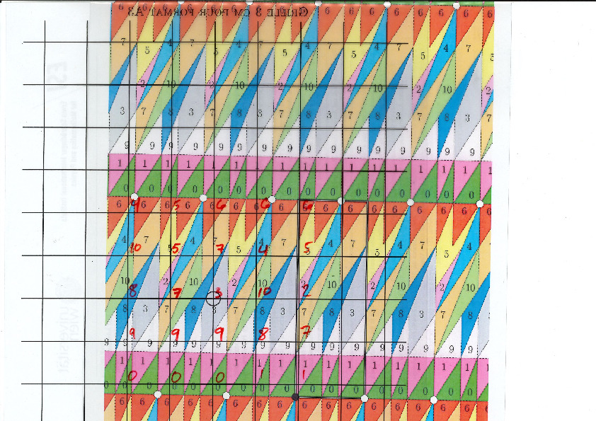
Each point of the lattice can be associated to an index from 0 to 10 according to which polygon of the partition it falls in. This defines a configuration of indices associated to each integer coordinate:
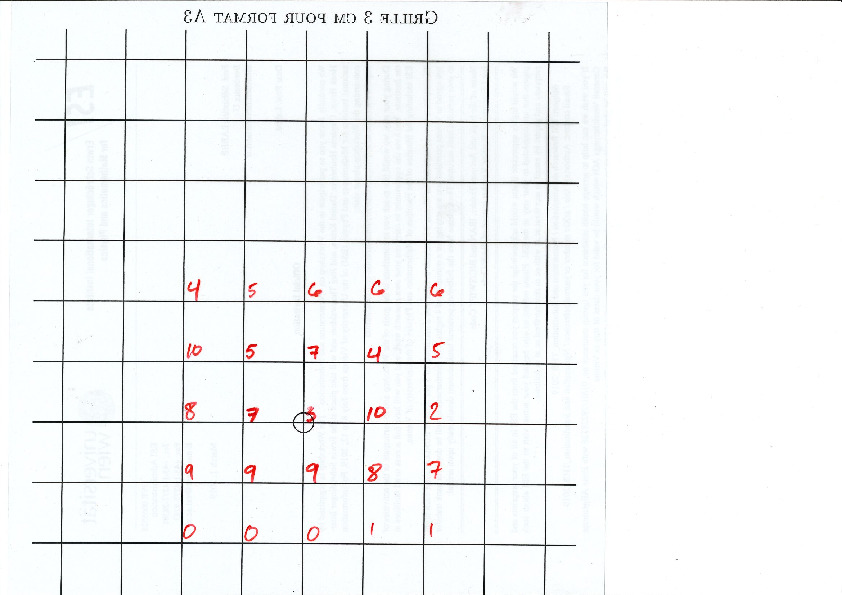
This procedure can be done all the way up to infinity. The chosen placement of the lattice defines a valid tiling of the plane with Jeandel-Rao tiles!

Since the size of the fundamental domain of the polygonal partition is irrational (width is golden mean, height is golden mean + 3, while the distance between two parallel gridlines is 1 unit), the generated configuration must be non-periodic.
It was a pleasure for me to do illustrate this to Emmanuel Jeandel during the workshop Multidimensional symbolic dynamics and lattice models of quasicrystals at CIRM in April 2024 in Marseille.
Do it yourself
Here are the files allowing to reproduce this experiment:
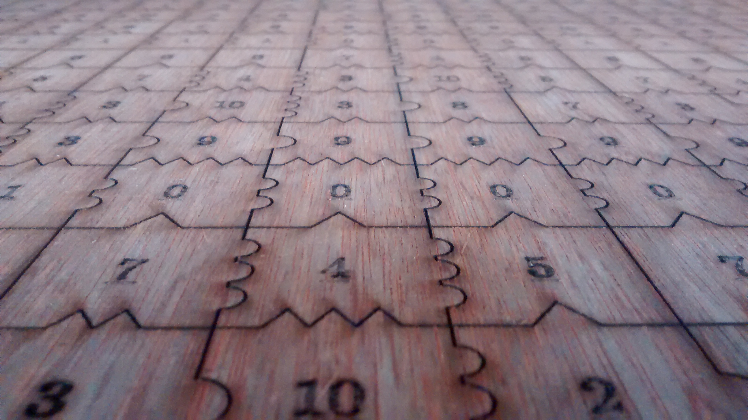
- A 33 x 19 rectangular valid patch of 627 tiles to use to cut a 1 meter x 60 cm wooden flat sheet (in svg format for laser cutting, pieces should have a side length of exactly 3 cm after the operation)
- The polygonal partition to be printed on a A3 paper (1 unit = 3 cm)
- The lattice \(\mathbb{Z}^2\) represented by gridlines 3cm apart to be printed on A4 paper (1 unit = 3 cm)
- A one-page Jeandel-Rao tiling solver tutorial
- A two-page document gathering the tutorial + partition (A4 paper format)
Alternate files for laser cutting the tiles
I first cut those tiles in August 2018 before a conference in Durham with the help of David Renault. We made more of them in June 2019. Each time David does some changes to the file that I provide to him with InkScape. Here are three alternate files for laser cutting the tiles.
Frequency of tiles
The frequency of tiles in a Jeandel-Rao tilings is computed below from the relative area in the associated polygonal partition. Tile #2 is the least frequent (around 2.55%) while tile #7 is the most frequent (around 15%):
sage: from slabbe.arXiv_1903_06137 import jeandel_rao_wang_shift_partition
sage: P0 = jeandel_rao_wang_shift_partition()
sage: V = P0.volume()
sage: tile_frequency = {a:v/V for (a,v) in P0.volume_dict().items()}
sage: rows = [(a, tile_frequency[a], tile_frequency[a].n(digits=3)) for a in range(11)]
sage: table(rows, header_row=['tile', 'frequency', 'frequency (numerical approx)'])
  tile   frequency           frequency (numerical approx)
├──────┼───────────────────┼──────────────────────────────┤
  0      -1/22*phi + 2/11    0.108
  1      -1/22*phi + 2/11    0.108
  2      9/22*phi - 7/11     0.0255
  3      -1/22*phi + 2/11    0.108
  4      2/11*phi - 5/22     0.0669
  5      -5/11*phi + 9/11    0.0828
  6      -1/22*phi + 2/11    0.108
  7      -3/11*phi + 13/22   0.150
  8      2/11*phi - 5/22     0.0669
  9      -1/22*phi + 2/11    0.108
  10     2/11*phi - 5/22     0.0669
When I construct a bag of 50 tiles of the Jeandel-Rao tiles, I follow the above tile frequencies. It yields:
sage: [(tile_frequency[a]*52).n(digits=3) for a in range(11)]
[5.63, 5.63, 1.33, 5.63, 3.48, 4.30, 5.63, 7.78, 3.48, 5.63, 3.48]
sage: [round(a) for a in _]
[6, 6, 1, 6, 3, 4, 6, 8, 3, 6, 3]
sage: sum(_)
52
Discussion
The construction of valid tilings with Jeandel-Rao tiles from a polygonal partition is a generalization of a well-known phenomenon in one dimension, namely, the fact that Sturmian sequences of complexity \(n+1\) are coded by irrational rotations. For example, here is an easy way to construct Sturmian sequences using a partition of the line into two intervals of different lengths. Similarly as above, every point from a set of equidistanced points is coded by letter A or B according to which of the two intervals it falls in.
The question that one may ask is whether all Jeandel-Rao tilings can be constructed from such a starting point in the partition. For Sturmian sequences, the answer is yes and the starting point can be described using the Ostrowski numeration system and the continued fraction expansion of the slope defined from the ratio of frequencies of the letters in the sequence. In one dimension, the proof is thus based on the desubstitution of Sturmian sequences on the one hand, and the Rauzy induction of irrational rotations on the other hand.
The same approach can be performed for Jeandel-Rao tilings using 2-dimensional desubstitution of Wang tilings and 2-dimensional Rauzy induction of toral \(\mathbb{Z}^2\)-rotations. Surprisingly, the two totally different methods applied on two completely different objects lead to the same sequence of eventually periodic 2-dimensional substitutions. Thus, every Jeandel-Rao tiling that can be desubstituted indefinitely can be constructed from the coding of some starting point in the polygonal partition.
Unfortunately, not all Jeandel-Rao tilings can be desubstituted indefinitely because of the existence of a horizontal fault line breaking the substitutive structure. Some configuration have a biinfinite horizontal row of the same tile labeled 0 in them. This allows to slide the lower half of configuration along the fault line and the configuration remains valid. A conjecture is that the remaining configurations are rare (of probability zero according to any shift-invariant probability measure). More precisely, I believe that all of the problematic ones can be described by a pair of starting points on the bottom segment of the polygonal partition. During the sabbatical year of Casey Mann and Jennifer Mcloud-Mann in Bordeaux in 2019-2020, we tried hard to prove that conjecture without success. It seems to be a difficult problem. Instead we described the nonexpansive directions in Jeandel-Rao tilings which reminds of the behavior of Penrose tilings with respect to Conway worms, their resolutions and essential holes (annulus of tiles which can be completed uniquely outside of the annulus, but not inside).
Aperiodic tilings related to the Metallic mean
The structure of Penrose aperiodic tilings, Jeandel-Rao aperiodic tilings and the new aperiodic hat monotile are all related to the golden mean. Do all aperiodic tilings need to be related to the golden ratio? What other numbers can be achieved?
During the conference at CIRM, I presented my newest result split into two parts: for every positive integer \(n\), there exists an aperiodic set of \((n+3)^2\) Wang tiles whose tiling structure is associated to the \(n\)-th metallic mean number, that is, the positive root of the polynomial \(x^2-nx-1\). This new discovery extends the knowledge we have on aperiodic tilings beyond the omnipresent golden ratio. The talk was recorded on youtube and the written notes are available here.
Jean-René Chazottes et Marc Monticelli
During the conference at CIRM, I met Jean-René Chazottes and Marc Monticelli. They made me know about their interactive online books, the outreach mathemarium website and its online experiments. Also, the Open-Fabrik-Maths fablab in Nice, including some experiments involving aperiodic Wang tilings.
Comment faire (et ne pas faire) un horaire pour un pool de 4 équipes
21 février 2024 | Mise à jour: 27 février 2024 | Catégories: ultimate | View CommentsTexte mis à jour le 27 février 2024
Dans ce texte, nous allons discuter des différentes manières de faire (et de ne pas faire) l'horaire d'un pool de 4 équipes dans un tournoi d'ultimate. Pour simplifier les choses, nous allons supposer que deux terrains sont disponibles pour faire jouer les 4 équipes en même temps et que tous les matchs du pool seront jouées sur une même journée. On suppose aussi qu'il existe un préclassement des équipes de 1 à 4 (1 étant la meilleure équipe, et 4 étant l'équipe présumée la plus faible).
Un peu de théorie
Tout d'abord, faisons un peu de théorie. Nous désirons respecter les trois Principes de base suivants:
- Principe no 1: Terminer avec les matchs les plus importants
- Principe no 2: Commencer avec les matchs les moins importants
- Principe no 3: Terminer avec le match le plus important
Pourquoi veut-on ces principes? Simplement parce que les équipes ne sont pas à leur meilleur potentiel en début de journée. Il est préférable de mesurer les équipes impliquées dans un match important le plus possible en fin de journée ou fin de pool.
Les matchs les plus importants sont les matchs entre des équipes préclassées proches une de l'autre (1 v 2, 2 v 3, 3 v 4). Les matchs les moins importants sont les matchs entre équipes préclassées loin une de l'autre (1 v 3, 2 v 4, 1 v 4).
Aussi, on dira que le match le plus important du pool sera celui qui fait intervenir la dernière équipe à être sélectionnée pour l'étape suivante et la meilleure équipe qui se fait éliminer du championnat. Par exemple, si seules les deux meilleures équipes passent en quart-de-finale (comme en Coupe du monde de football), alors le match le plus important du pool est le match 2 v 3. Si seule la meilleure équipe du pool est sélectionnée pour l'étape suivante, alors le match le plus important est le match 1 v 2. Si seule la dernière équipe est éliminée du championnat après le pool (comme pendant les Championnats canadiens d'ulimate), alors le match 3 v 4 est le match le plus important du pool.
Attention avant de vouloir adapter les principes discuté ici pour des pools plus grands impliquant 6 équipes et plus où les matchs seront répartis sur plus d'une journée. La question se pose alors de savoir si la priorité est de faire jouer les matchs les plus importants à la fin du pool ou à la fin de la première journée. Cela est un autre sujet: continuons plutôt de considérer le cas d'un pool de 4 équipes.
Option 1
La première option à laquelle on peut penser est de faire jouer les équipes dans l'ordre suivant. On se met dans la peau de la meilleure équipe, et on veut la faire jouer contre des équipes de plus en plus forte au fur et à mesure que la journée avance:
| Ronde | Terrain 1 | Terrain 2 |
|---|---|---|
| Ronde 1 | 1 v 4 | 2 v 3 |
| Ronde 2 | 1 v 3 | 2 v 4 |
| Ronde 3 | 1 v 2 | 3 v 4 |
Sans savoir quel est le match le plus important, on peut déjà dire que c'est déjà un très mauvais choix de format pour deux raisons:
- (Principe no 1 non respecté) Le match 2 v 3 est un match important et ne devrait pas être joué pour commencer le pool.
- (Principe no 2 non respecté) Les matchs 1 v 3 et 2 v 4 sont moins importants et devraient être joués en début de pool.
C'est ce format que la FFFD a choisi comme format de tournoi pour les pools de 4 équipes pour les Championnat de France Beach Mixte N1 N2 et N3 du 23-24 septembre 2023. Le format de la FFFD est fait de 4 pools de 4 équipes et seuls les top 2 de chaque pool sont qualifiées pour l'étape suivante (quart-de-finales). Cela signifie que le match le plus important est le match 2 v 3, qui devrait donc être joué à la fin du pool (Principe no 3 non respecté). Or, c'est le match qui est joué en premier le samedi matin. Bref, ce n'est pas idéal, car le format décide avec haute probabilité qui va jouer dans le top 8 au tout premier match du samedi matin alors que les équipes ne sont pas à leur plein potentiel.
Option 2
L'option classique d'un pool de 4 équipes est le format suivant:
| Ronde | Terrain 1 | Terrain 2 |
|---|---|---|
| Ronde 1 | 1 v 3 | 2 v 4 |
| Ronde 2 | 1 v 4 | 2 v 3 |
| Ronde 3 | 1 v 2 | 3 v 4 |
On a que
- Le Principe 2 est respecté, car on commence avec les matchs les moins importants.
- Le Principe 1 est respecté, car on termine avec les matchs les plus importants (2 v 3, puis 1 v 2 et 3 v 4).
- Le Principe 3 est respecté si le match le plus important est le match 1 v 2 ou 3 v 4.
C'est le format de base recommandé par USA Ultimate pour 4 équipes dans le manuel des formats de tournois d'ultimate qui existe depuis 1993.
Observons que l'option 2 est compatible avec l'existence d'une 4e ronde de matchs de croisement après la phase de pools et avant la phase à élimination directe. Il s'agit de croiser les équipes terminant en 2e et 3e position dans les pools distincts. Par exemple, avec quatre pools A-B-C-D, les matchs de croisement (aussi appelés pré-quarts dans ce cas-ci) sont A2 v D3, A3 v D2, B2 v C3, B3 v C2 dont les gagnants se retrouvent en quart-de-finales contre les gagnants des pools.
Les matchs de croisement permettent de gérer la situation où on a trois équipes fortes qui se retrouvent dans le même pool. Le match de croisement permet à une équipe qui termine 3e d'un pool de tenter de gagner contre une équipe qui a terminé 2e dans un autre pool pour se qualifier pour l'étape suivante.
Avec des matchs de croisement 2e v 3e, seule la 4e équipe est éliminée à la fin des matchs de pool. Le match 3 v 4 du pool est donc le match le plus important. Cette situation est donc compatible avec l'option 2 (Principe no 3 respecté).
Option 3
Lorsque seules 2 équipes sur 4 sont qualifiées pour l'étape suivante, alors le match 2 v 3 devient le match le plus important du pool. En ce sens, l'option 2 ci-haut ne respecte pas le Principe no 3, car le match 2 v 3 est joué en deuxième ronde.
Dans ce cas, il est préférable de procéder ainsi:
| Ronde | Terrain 1 | Terrain 2 |
|---|---|---|
| Ronde 1 | 1 v 3 | 2 v 4 |
| Ronde 2 | 1 v 2 | 3 v 4 |
| Ronde 3 | 1 v 4 | 2 v 3 |
On a que:
- Le Principe 2 est respecté, car on commence avec les matchs les moins importants.
- Le Principe 1 est quasiment respecté, car on termine avec les matchs les plus importants (1 v 2 et 3 v 4 puis 2 v 3).
- Le Principe 3 est respecté, car on termine avec le match le plus important (2 v 3).
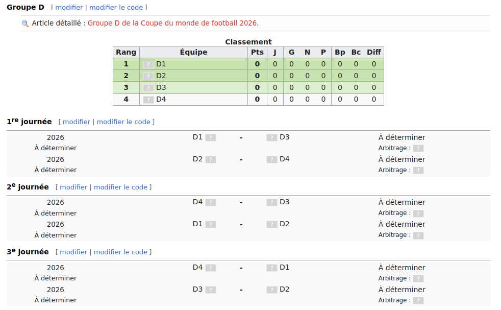
C'est ce format que la FIFA choisit lors de la Coupe du monde pour les pools de 4 équipes où le match 2 v 3 est le match le plus important du pool. Voici une copie écran de la page Wikipédia sur la Coupe du monde de football 2026:
Option 4
Il existe une 4e option proposée dans le manuel de USA Ultimate qui mérite d'être mentionnée:
| Ronde | Terrain 1 | Terrain 2 |
|---|---|---|
| Ronde 1 | 1 v 3 | 2 v 4 |
| Ronde 2 | gagnant v perdant | gagnant v perdant |
| Ronde 3 | match restant | match restant du tournoi à la ronde |
Lorsque le préclassement est incertain, ce format augmente les chances que les équipes invaincues se rencontrent en troisième ronde. Si le préclassement est respecté dans les matchs, alors l'option 4 est équivalente à l'option 2.
Conclusion
Si vous organisez un tournoi, merci de ne pas réinventer la roue. Les formats de tournois ont été beaucoup étudiés dans le passé (USA Ultimate, FIFA, etc.). Merci de consulter par exemple le manuel des formats des tournois de USA Ultimate ou ce qui se passe dans les autres fédérations et à l'international.
Pour ce qui est de l'horaire des pools de 4 équipes, voici mes recommandations
- si une ou trois équipes du pool sont qualifiées pour l'étape suivante, alors je recommande d'utiliser l'option 2: le format classique recommandé dans le manuel des formats de tournoi de USA Ultimate.
- si deux équipes du pool sont qualifiées pour l'étape suivante, alors je recommande d'utiliser l'option 3: le format des pools de la Coupe du monde de football de la FIFA.
- dans tous les cas, je recommande de proscrire l'option 1.
« Previous Page -- Next Page »
Propulsé par Blogofile
S'abonner au Flux RSS
et aux Commentaires.

This work by Sébastien Labbé is licensed under a Creative Commons Attribution-ShareAlike 4.0 International License.