Sébastien Labbé

La Fédération québécoise d'ultimate est en train de concevoir son propre modèle de développement de l'athlète, modèle que chaque fédération doit avoir. Dans ce texte, je transmettrai quelques-unes des réflexions que j'ai sur le sujet. Bien sûr, mes réflexions sont limitées et proviennent en grande partie d'une seule source, car ce n'est pas du tout mon sujet de recherche.

Savoir comment développer les meilleurs athlètes est une très grande question et je suis sûr que les réponses qu'on y apporte évolue au fil des années selon les expériences qui s'acquièrent et surtout suites aux erreurs qui sont faites et ce dans tous les sports. Ainsi, je pense que la fédération doit s'appuyer sur ce qui a de mieux. Or, qui possède cette expertise? Qui sont les experts?

À la conférence annuelle d'Ultimate Canada tenue en novembre 2011 à Québec (dont j'avais fait un résumé), Charles Cardinal était le conférencier invité et il avait fait une très bonne présentation. Pour ma part, c'est à ce moment-là que j'ai été sensibilisé pour la première fois à cette question. M. Cardinal, qui avait été longtemps entraîneur de volleyball, nous disait de profiter du fait que nous sommes un jeune sport pour ne pas refaire les erreurs du passé. Cela signifie que nous avons aujourd'hui la responsabilité de connaître quelles sont les erreurs du passé.

Je me souviens qu'il parlait des entraîneurs qui visaient la victoire pour des équipes d'adolescents. Oui, ils obtenaient la victoire. Ils étaient champions québécois, peut-être même champions canadiens à 15 ans, mais ce sont des joueurs qui à 17-18-19 ans abandonnaient le sport, car on les avaient écoeurés pendant l'adolescence.

Un autre exemple dont il avait parlé était à propos des jeunes qui ont une poussée de croissance tardive. Ces jeunes sont souvent mis de côté dans les sélections des équipes élites adolescentes. Par contre, des recherches montrent que ces jeunes peuvent atteindre des niveaux encore plus élevés dans la vingtaine, d'où l'importance de ne pas les mettre de côté.

Il a cité un nombre encore plus grand d'erreurs commises par le passé à ne pas refaire. J'ai réussi à en trouver une liste (Les problèmes dans le sport) sur le site de Au Canada, le sport c'est pour la vie, organisation qui semble avoir réuni les experts que nous cherchons. Ce site contient une foule d'informations dont les modèles de développement à long terme de l'athlète pour plusieurs sports (Consulter nos ressources > Modèles de DLTA canadiens propres à chaque sport).

Sur le même site, on y décrit les 7 stades du Développement à long terme de l’athlète (DLTA) sur lequel le modèle de développement de l'athlète à l'ultimate doit se baser:

• Stade 1 : Enfant actif (0-6 ans)
• Stade 2 : S’amuser grâce au sport (filles 6-8, garçons 6-9)
• Stade 3 : Apprendre à s’entraîner (filles 8-11, garçons 9-12)
• Stade 4 : S’entraîner à s’entraîner (filles 11-15, garçons 12-16)
• Stade 5 : S’entraîner à la compétition (filles 15-21, garçons 16-23)
• Stade 6 : S’entraîner à gagner (filles 18+, garçons 19+)
• Stade 7 : Vie active (participants de tout âge)

Après la conférence de M. Cardinal, à notre table de 5 ou 6 personnes, on devait discuter du contenu propre à l'ultimate dans chacun des stades. Cette discussion m'a fait comprendre que nous sommes aussi capables, à l'ultimate comme dans les autres sports, de faire des erreurs (selon mon opinion personnel). En effet, une des personnes à notre table expliquait qu'en tant qu'entraîneur, il obligerait ses joueurs à lancer que des revers et des lancers droits et interdirait les lancers marteau et autres lancers particuliers. À mon avis, c'est une erreur. On ne veut pas développer des athlètes à l'image de notre génération. On veut développer des athlètes qui seront les meilleurs pour pratiquer l'ultimate. Or dans les règlements de l'ultimate, il n'est pas fait mention de la manière de lancer le disque. Alors pourquoi ajouter de telles interdictions? Au contraire, j'aimerais que la prochaine génération ne possède pas notre handicap et puisse lancer le disque de toutes les façons!

Je désire réitérer un conseil de M. Cardinal au sujet qu'il faut absolument miser sur l'aspect esprit du jeu et communautaire, deux valeurs essentielles à l'ultimate, dans notre approche de développement de l'athlète.

Finalement, je désire terminer en transmettant les réflexions que j'ai eues depuis la conférence de M. Cardinal, c'est-à-dire depuis un an et demi. Je n'ai pas beaucoup d'expérience sur le développement des jeunes joueurs juniors d'ultimate et à quel moment serait-il propice d'apprendre quoi. Par contre, je suis capable de repérer les bons joueurs et les mauvais joueurs autour de moi une fois grands. Ainsi, c'est sous cet angle maintenant que je réfléchis aux habiletés qui doivent être développées en jeune âge et les habiletés pour lesquelles il n'est pas trop tard de développer dans une équipe senior pendant une ou deux saisons pour atteindre un objectif comme gagner les Championnats canadiens.

Le gouvernement du Québec me déçoit grandement ces jours-ci lorsque je lis dans les nouvelles que nous continuerons de payer pour des logiciels propriétaires alors qu'il existe, en 2013, des logiciels libres qui sont tout aussi bon sinon mieux.

• Québec : les logiciels libres écartés?, Canoe, 11 février 2013
• Un centre d'expertise en logiciel libre, mais un contrat à Microsoft, Radio-Canada, 18 mars 2013
• Québec adopte deux décrets contre le logiciel libre, Le Devoir, 29 mars 2013

Pourtant, le parti au pouvoir sait bien qu'il commet une erreur. En effet, il l'affirmait lui-même l'an dernier à pareil date:

• Québec doit «réduire sa dépendance à Microsoft», dit le PQ, La Presse, 30 mars 2012

Doit-on rappeler les enjeux?

Pour les logiciels libres dans nos écoles

Pour éviter de payer pour qu'une génération complète de citoyens du Québec ne connaissent et ne savent utiliser que des logiciels propriétaires obligeant ainsi toute la société (dont les entreprises) à payer eux aussi chers de licences pour des logiciels.

Pour les logiciels libres au gouvernement

Le gouvernement du Québec ne doit pas payer des millions de dollars (sinon milliards) pour des logiciels propriétaires alors qu'il existe des logiciels équivalents libres et gratuits.

Maîtres chez nous version 2013: pour une expertise québécoise en logiciels libres

La dépendance face à des entreprises étrangères doit être remplacée par une autonomie québécoise et par le développement d'une expertise québécoise en logiciels libres. Nous ne sommes jamais aussi bien servis que par nous-mêmes!

Parce que nous ne sommes plus en 1993

Nous ne sommes plus en 1993. Nous sommes en 2013. Écrire un logiciel de traitement texte, ce n'est pas compliqué. Ce n'est plus nécessaire de payer pour cela! Le logiciel libre existe et c'est gratuit.

Pour le métier de mécanicien automobile, c'est être pour le logiciel libre

Mon père, mon grand-père et mon arrière-grand-père sont et ont été mécaniciens automobiles depuis 1954. Ils ont toujours aimé observer les mécanismes afin de les comprendre, repérer les problèmes et trouver des solutions. Ainsi, ma famille comprendra bien la comparaison suivante.

Si un logiciel était une voiture, un logiciel propriétaire serait une voiture dont l'ouverture du capot serait interdite par la loi et passible de poursuite, dont la réparation ou la modification serait aussi interdite et où les mécaniciens automobiles et autres réparateurs seraient considérés des pirates bandits.

Un logiciel libre permet d'être ouvert, observé, analysé, compris, modifié, amélioré. Je pense que les usagers de logiciels méritent la liberté et devraient bénéficier des informaticiens comme on bénéficie des mécaniciens pour réparer une voiture.

Parce que la souveraineté, ce n'est pas juste un mot

Un parti politique qui prolonge notre dépendance aux logiciels propriétaires ne peut pas prétendre défendre l'indépendance et rester crédible.

Qu'est-ce que le logiciel libre

Un logiciel libre, en plus d'être gratuit, garanti les 4 libertés suivantes:

0. Liberté d'utilisation (gratuité)
1. Liberté de regarder le code
2. Liberté de modifier le code
3. Liberté de redistribuer le logiciel possiblement modifié

Qui veut payer pour avoir moins de libertés?

Utiliser un logiciel propriétaire, c'est donc payer pour avoir moins de libertés. Qui est prêt à faire ça?

Pour en savoir plus

Voici un texte ainsi qu'une entrevue de Richard Stallman permettant d'en savoir plus sur les logiciels libres.

• Mesures à la portée des gouvernements pour promouvoir le logiciel libre
• Copyright et mondialisation à l'âge des réseaux informatiques

(NEW: See also the demo I made at the Sage Paris group meeting in March 2014.)

Ticket #12719 (Upgrade to IPython 0.13) was merged into sage-5.7.beta1. This took a lot of energy (see the number of comments in the ticket and especially the number of patches and dependencies). Big thanks to Volker Braun, Mike Hansen, Jason Grout, Jeroen Demeyer who worked on this since almost one year. Note that in December 2012, the IPython project has received a $1.15M grant from the Alfred P. Sloan foundation, that will support IPython development for the next two years. I really like this IPython sage command line interface so it is really good news!

The IPython notebook

Since version 0.12 (December 21 2011), IPython is released with its own notebook. The differences with the Sage Notebook are explained by Fernando Perez, leader of IPython project, in the blog post The IPython notebook: a historical retrospective he wrote in January 2012. One of the differences is that the IPython Notebook run in its own directory whereas each cell of the Sage Notebook lives in its directory. As William Stein says in the presentation Browser-based notebook interfaces for mathematical software - past, present and future he gave last December at ICERM, there are plenty of projects and directions these days for those interfaces.

In May 2012, I tested the same ticket which was to upgrade to IPython 0.12 at that time. Today, I was curious to test it again.

First, I installed sage-5.7.beta4:

./sage -version
Sage Version 5.7.beta4, Release Date: 2013-02-09

Install tornado:

./sage -sh
easy_install-2.7 tornado

[update March 6th, 2014] Note that some linux user have to install libssl-dev before tornado:

sudo apt-get install libssl-dev

Install zeromq and pyzmq:

./sage -i zeromq
./sage -i pyzmq

Start the ipython notebook:

./sage -ipython notebook
[NotebookApp] Using existing profile dir: u'/Users/slabbe/.sage/ipython-0.12/profile_default'
[NotebookApp] Serving notebooks from /Users/slabbe/Applications/sage-5.7.beta4
[NotebookApp] The IPython Notebook is running at: http://127.0.0.1:8888/
[NotebookApp] Use Control-C to stop this server and shut down all kernels.

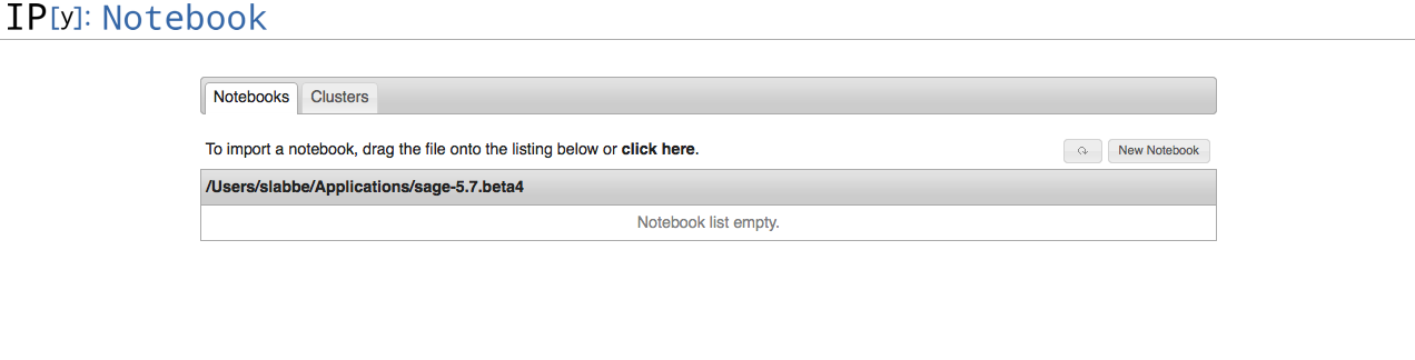
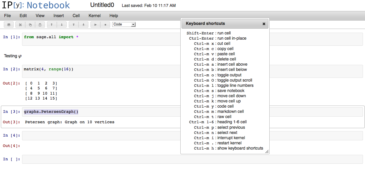
Create a new notebook. One may use sage commands by adding the line from sage.all import * in the first cell.

The next things I want to look at are:

• Test the conversion of files from .py to .pynb.
• Test the conversion of files from .rst to .pynb.
• Test the qtconsole.
• Test the parallel computing capacities of the IPython.

Since Sage Days 20 at Marseille held in January 2010, I have been doing the same example over and over again each time I showed someone else how object oriented coding works in Python: using fruits, strawberry, oranges and bananas.

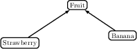
Here is my file: fruit.py. I use to build it from scratch by adding one line at a time using attach command to see what has changed starting with Banana class, then Strawberry class then Fruit class which gathers all common methods.

This time, I wrote the complete documentation (all tests pass, coverage is 100%) and followed Sage coding convention as far as I know them. Thus, I hope this file can be useful as an example to explain those coding convention to newcomers.

One may check that all tests pass using:

$ sage -t fruit.py
sage -t  "fruit.py"
[3.7 s]

----------------------------------------------------------------------
All tests passed!
Total time for all tests: 3.8 seconds

One may check that documentation and doctest coverage is 100%:

$ sage -coverage fruit.py
----------------------------------------------------------------------
fruit.py
SCORE fruit.py: 100% (10 of 10)
----------------------------------------------------------------------

This message is about differences between a Python function and a symbolic function. This is also explained in the Some Common Issues with Functions page in the Sage Tutorial.

In Sage, one may define a symbolic function like:

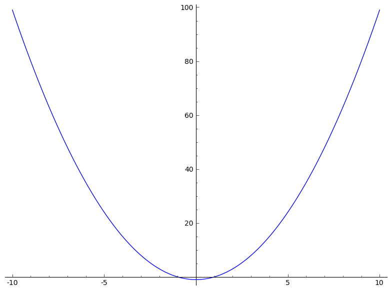
sage: f(x) = x^2-1

And draw it using one the following way (both works):

sage: plot(f, (x,-10,10))
sage: plot(f(x), (x,-10,10))

Here both f and f(x) are symbolic expressions:

sage: type(f)
<type 'sage.symbolic.expression.Expression'>
sage: type(f(x))
<type 'sage.symbolic.expression.Expression'>

although there are different:

sage: f
x |--> x^2 - 1
sage: f(x)
x^2 - 1

Now if f is a Python function defined with a def statement:

sage: def f(x):
....:     if x>0:
....:         return x
....:     else:
....:         return 0

It is really a Python function:

sage: f
<function f at 0xb933470>
sage: type(f)
<type 'function'>

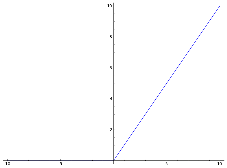
As above, one can draw the function f:

sage: plot(f, (x,-10,10))

But be carefull, drawing f(x) will not work as expected:

sage: plot(f(x), (x,-10,10))

Why? Because, the python function f gets evaluated on the variable x and this may either raise an exception depending on the definition of f or return some result which might not be a symbolic expression. Here f(x) gets always evaluated to zero because in the definition of f, bool(x > 0) returns False:

sage: x
x
sage: bool(x > 0)
False
sage: f(x)
0

Hence the following constant function is drawn:

sage: plot(0, (x,-10,10))

which is not what we want.