Basic Definitions

Let \(\mathbb{L}^d=(\mathbb{Z}^d,\mathbb{E}^d)\) be the hypercubic lattice. Let \(p\in[0,1]\). Each edge \(e\in \mathbb{E}^d\) is designated either open with probability \(p\), or closed otherwise, different edges receiving independant states. For \(x,y\in \mathbb{Z}^d\), we write \(x \leftrightarrow y \) if there exists an open path joining \(x\) and \(y\). For \(x\in \mathbb{Z}^d\), we consider the open cluster \(C_x\) containing \(x\) : \[ C_x = \{y \in \mathbb{Z}^d : x \leftrightarrow y \}. \] The percolation probability \(\Theta(p)\) is given by \[ \Theta(p) = P_p(\vert C_0\vert=\infty). \] Finally, the critical probability is defined as \[ p_c = \sup\{p : \Theta(p) = 0 \}. \] The question is to compute \(p_c\). Results in the Chapter give lower bound and upper bound for \(p_c\). Many problems are still open like the one claiming that \(\Theta(p_c) = 0\) for all \(d\geq 2\): it is known only for \(d=2\) and \(d\geq 19\) according to a remark in the chapter.

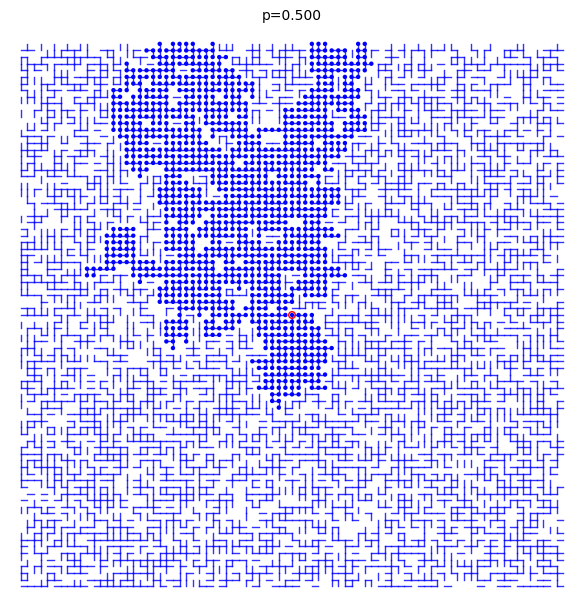
Some samples when p=0.5

A bond percolation sample inside the box \(\Lambda(m)=[-m,m]^d\) when \(p=0.5\) and \(d=2\):

sage: S = BondPercolationSample(p=0.5, d=2)
sage: S.plot(m=40, pointsize=10, thickness=1)
Graphics object consisting of 7993 graphics primitives
sage: _.show()

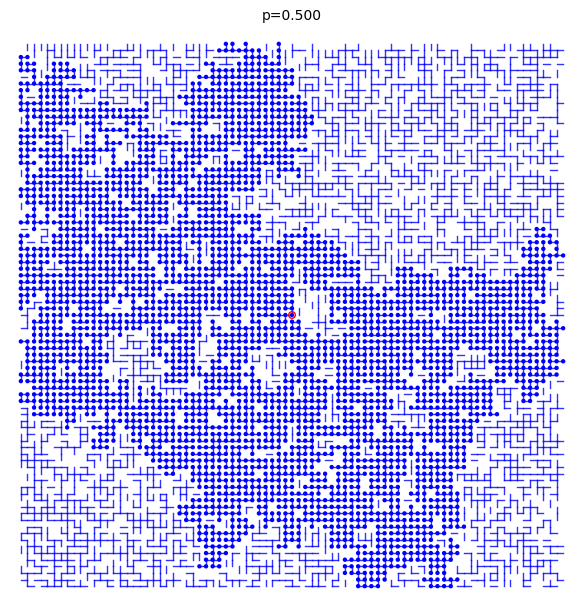
Another time gives something different:

sage: S = BondPercolationSample(p=0.5, d=2)
sage: S.plot(m=40, pointsize=10, thickness=1)
Graphics object consisting of 10176 graphics primitives
sage: _.show()

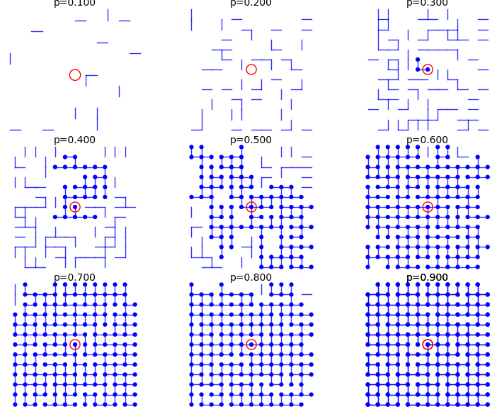
Some samples for ranges of values of p

From p=0.1 to p=0.9:

sage: percolation_graphics_array(srange(0.1,1,0.1), d=2, m=5)

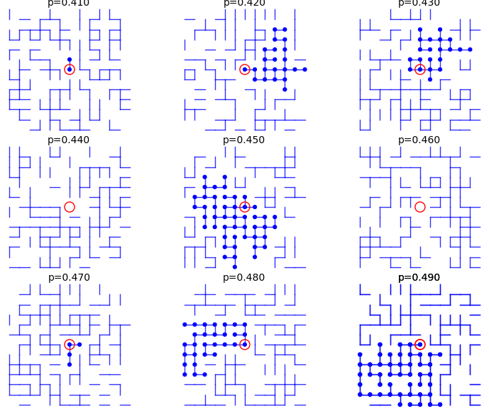
From p=0.41 to p=0.49:

sage: percolation_graphics_array(srange(0.41,0.50,0.01), d=2, m=5)

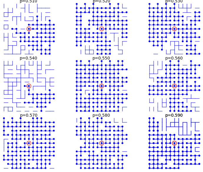
From p=0.51 to p=0.59:

sage: percolation_graphics_array(srange(0.51,0.60,0.01), d=2, m=5)

Upper bound and lower bound for percolation probability \(\Theta(p)\)

In every case, we have the following upper bound for the percolation probability: \[ \Theta(p) = \mathbb{P}_p(\vert C_0\vert=\infty) \leq \mathbb{P}_p(\vert C_0\vert > 1) = 1 - \mathbb{P}_p(\vert C_0\vert = 1) = 1 - (1-p)^{2d}. \] In particular, if \(p\neq 1\), then \(\Theta(p)<1\). In Sage, define the upper bound:

sage: p,n = var('p,n')
sage: d = var('d')
sage: upper_bound = 1 - (1-p)^(2*d)

Also, from Equation (3.8), we have the following lower bound: \[ \Theta(p) \geq 1 - \sum_{n=4}^{\infty} n (4(1-p))^n. \]

In Sage, define the lower bound:

sage: p,n = var('p,n')
sage: lower_bound = 1 - sum(n*(4*(1-p))^n,n,4,oo)
sage: lower_bound.factor()
-(3072*p^5 - 14336*p^4 + 26624*p^3 - 24592*p^2 + 11288*p - 2057)/(4*p - 3)^2

This is not defined when \(p=3/4\), but we are interested in the values in the interval \(]3/4,1]\). In particular, for which value of \(p\) is this lower bound strictly larger than zero:

sage: root = lower_bound.find_root(0.76, 0.99); root
0.8639366490304586

Let's now draw a graph of the lower and upper bound:

sage: U = plot(upper_bound(d=2),(0,1),color='red', thickness=3)
sage: L = plot(lower_bound,(0.86,1),color='green', thickness=3)
sage: G = U + L
sage: G += point((root, 0), color='red', size=20)
sage: lower = r"$1-\sum_{n=4}^{\infty} n4^n(1-p)^n$"
sage: upper = r"$1 -(1-p)^{4}$"
sage: title = r"$1-\sum_{n=4}^{\infty} n4^n(1-p)^n\leq\Theta(p)\leq 1 -(1-p)^{2d}$"
sage: G += text(title, (.5, 1.05), color='black', fontsize=15)
sage: G += text(upper, (.3, 0.5), color='red', fontsize=20)
sage: G += text(lower, (.7, 0.5), color='green', fontsize=20)
sage: G += text("%.5f"%root,(0.88, .03), color='green', horizontal_alignment='left')
sage: G.show()

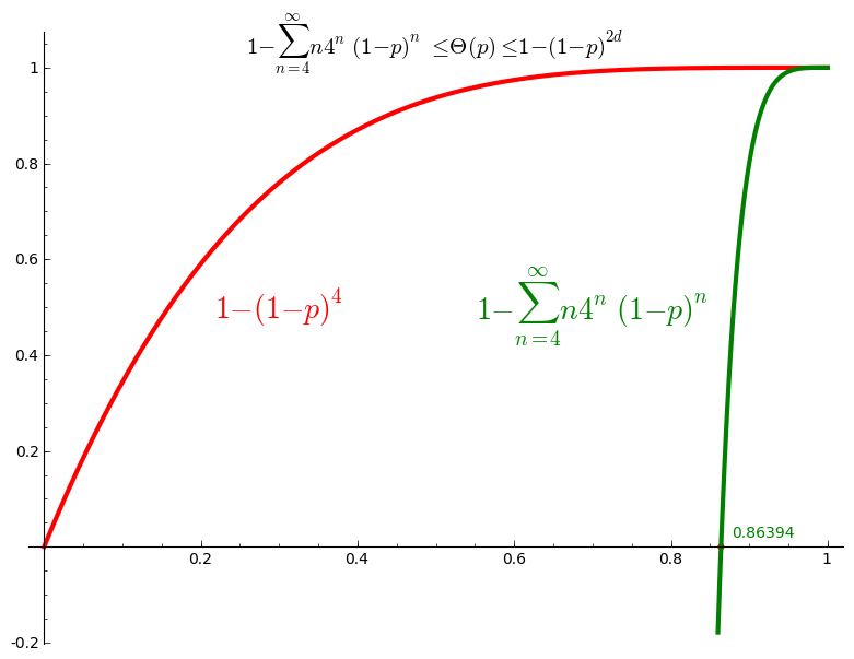
Thus we conclude that \(\Theta(p) >0\) for \(p>0.8639\) and thus \(p_c \leq 0.8639\).

Percolation probability - dimension 2

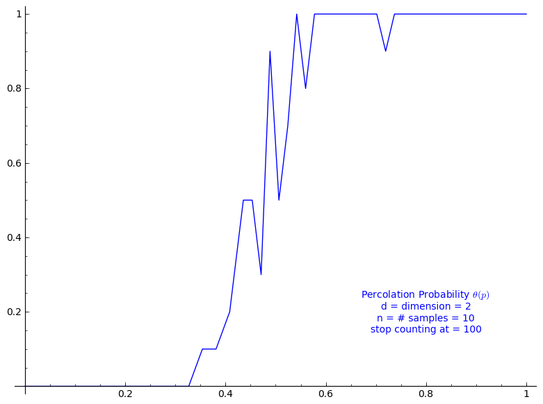
The code allows to define the percolation probability function for a given dimension d. It generates n samples and consider the cluster to be infinite if its cardinality is larger than the given stop value.

Here we use Sage adaptative recursion algorithm for drawing the plot of the percolation probability which finds the particular important intervals to ask for more values of the function. See help section of plot function for details. Because T might be long to compute we start with only 4 points.

When stop=100:

sage: T = PercolationProbability(d=2, n=10, stop=100)
sage: T.return_plot((0,1),adaptive_recursion=4,plot_points=4).show()

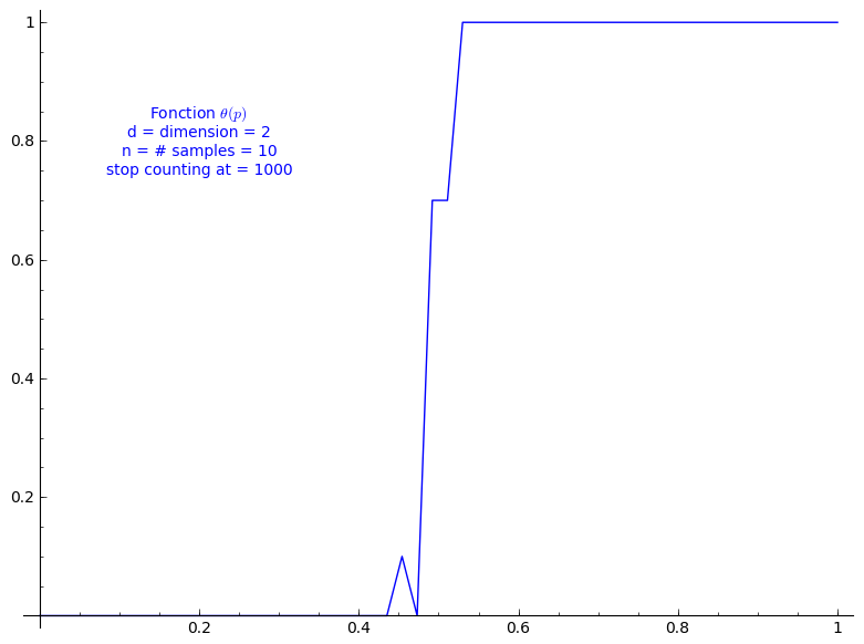
When stop=1000:

sage: T = PercolationProbability(d=2, n=10, stop=1000)
sage: T.return_plot((0,1),adaptive_recursion=4,plot_points=4).show()

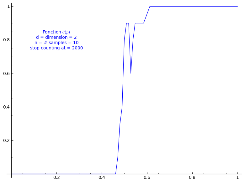
When stop=2000:

sage: T = PercolationProbability(d=2, n=10, stop=2000)
sage: T.return_plot((0,1),adaptive_recursion=4,plot_points=4).show()

Percolation probability - dimension 3

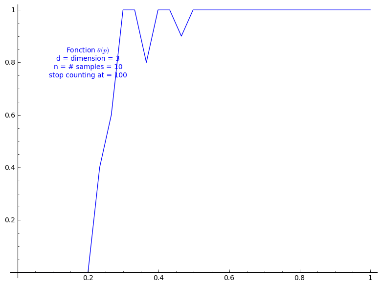
When stop=100:

sage: T = PercolationProbability(d=3, n=10, stop=100)
sage: T.return_plot((0,1),adaptive_recursion=4,plot_points=4).show()

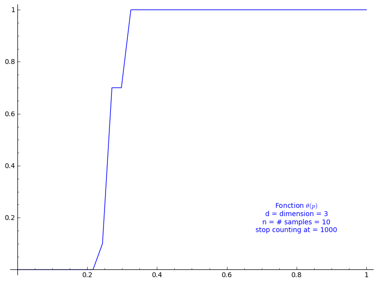
When stop=1000:

sage: T = PercolationProbability(d=3, n=10, stop=1000)
sage: T.return_plot((0,1),adaptive_recursion=4,plot_points=4).show()

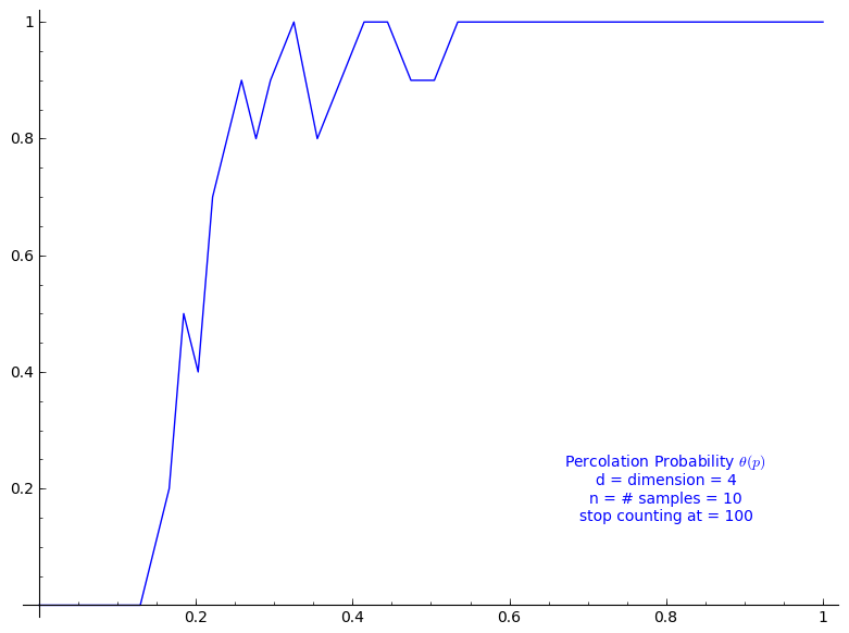
Percolation probability - dimension 4

When stop=100:

sage: T = PercolationProbability(d=4, n=10, stop=100)
sage: T.return_plot((0,1),adaptive_recursion=4,plot_points=4).show()

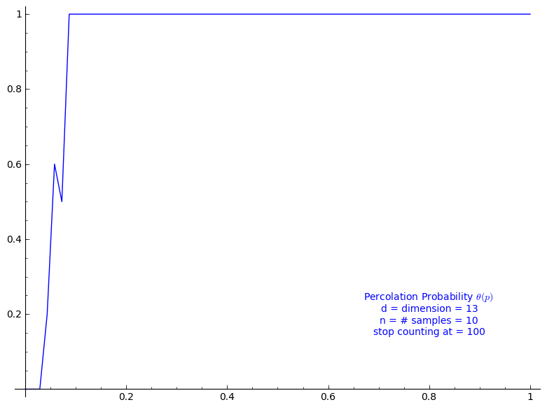
Percolation probability - dimension 13

When stop=100:

sage: T = PercolationProbability(d=13, n=10, stop=100)
sage: T.return_plot((0,1),adaptive_recursion=4,plot_points=4).show()

Theorem 3.2

Theorem 3.2 states that \(0 < p_c < 1\), but its proof does much more in fact. Following the computation we just did for Equation (3.8), we get for \(d=2\) \[ 0.3333 < \frac{1}{2d-1} \leq p_c \leq 0.8639 \] and for \(d=3\): \[ 0.2000 < \frac{1}{2d-1} \leq p_c \leq 0.8639 \] This allows to grasp the improvement brought later by Theorem 3.12.

Connective constant

Using the two following sequences of the On-Line Encyclopedia of Integer Sequences, one can evaluate the connective constant \(\kappa(d)\)

• A001411: Number of n-step self-avoiding walks on square lattice.
• A001412: Number of n-step self-avoiding walks on cubic lattice.

By taking the k-th root of of k-th term of A001411, we may give an approximation of \(\kappa(2)\):

sage: L = [1, 4, 12, 36, 100, 284, 780, 2172, 5916, 16268, 44100, 120292,
324932, 881500, 2374444, 6416596, 17245332, 46466676, 124658732, 335116620,
897697164, 2408806028, 6444560484, 17266613812, 46146397316, 123481354908,
329712786220, 881317491628]
sage: for k in range(1, len(L)): print numerical_approx(L[k]^(1/k))
4.00000000000000
3.46410161513775
3.30192724889463
3.16227766016838
3.09502148400370
3.03400133198980
2.99705187539871
2.96144397263395
2.93714926770637
2.91369345857619
2.89627439045790
2.87949308754677
2.86632078916860
2.85362749495679
2.84328447096562
2.83329615650289
2.82493415671599
2.81684125361654
2.80992368218258
2.80321554383456
2.79738645741910
2.79172363211806
2.78673687369245
2.78188437392354
2.77756387722633
2.77335345579129
2.76956977331575

By taking the k-th root of of k-th term of A001412, we may give an approximation of \(\kappa(3)\):

sage: L = [1, 6, 30, 150, 726, 3534, 16926, 81390, 387966, 1853886,
8809878, 41934150, 198842742, 943974510, 4468911678, 21175146054,
100121875974, 473730252102, 2237723684094, 10576033219614, 49917327838734,
235710090502158, 1111781983442406, 5245988215191414, 24730180885580790,
116618841700433358, 549493796867100942,2589874864863200574,
12198184788179866902, 57466913094951837030, 270569905525454674614]
sage: for k in range(1, len(L)): print numerical_approx(L[k]^(1/k))
6.00000000000000
5.47722557505166
5.31329284591305
5.19079831727404
5.12452137580198
5.06709510955294
5.02933019629493
4.99573287588832
4.97111339009676
4.94876680377358
4.93129192790635
4.91521453865211
4.90209314463520
4.88990167518413
4.87964724632057
4.87004597517131
4.86178722582108
4.85400655861169
4.84719703702142
4.84074902256992
4.83502763526502
4.82958688248615
4.82470487210973
4.82004549244633
4.81582557693112
4.81178552451599
4.80809774735294
4.80455755518719
4.80130435575213
4.79817388859565

Then, \(\kappa(2)\) would be something less than 2.769 and \(\kappa(3)\) would be something less than 4.798.

Theorem 3.12

Thus, we may evaluate the lower bound and upper bound given at Theorem 3.12. For dimension \(d=2\):

sage: k < 2.76956977331575
k < 2.76956977331575
sage: _ / (2.76956977331575  * k)
0.361066909970928 < (1/k)
sage: 1 - 0.361066909970928
0.638933090029072

The critical probability of bond percolation on \(\mathbb{L}^d\) with \(d=2\) satisfies \[ 0.3610 < \frac{1}{\kappa(2)} \leq p_c \leq 1 - \frac{1}{\kappa(2)} < 0.6389. \] If we look at the graph of the percolation probability \(\Theta(p)\) we did above for when \(d=2\), it seems that the lower bound is not far from \(p_c\). The lower bound 0.3610 is a small improvement to the simple one got from Theorem 3.2 (0.3333).

Similarly, for dimension \(d=3\):

sage: k < 4.79817388859565
k < 4.79817388859565
sage: _ / (4.79817388859565 * k)
0.208412621805310 < (1/k)

The critical probability of bond percolation on \(\mathbb{L}^d\) with \(d=3\) satisfies \[ 0.2084 < \frac{1}{\kappa(3)} \leq p_c \leq 1 - \frac{1}{\kappa(2)} < 0.6389. \] Again, if we look at the graph of \(\Theta(p)\) we did above for when \(d=3\), it seems that the lower bound 0.2084 is not far from \(p_c\). In this case, the lower bound 0.2084 is a rather small improvement to the lower bound from Theorem 3.2 (0.2000). It might be caused by a poor approximation of \(\kappa(3)\) from the above sequences of only 30 terms from the OEIS.