Introduction to Python/SageMath
27 juin 2023 | Catégories: sage, math | View CommentsOn Wednesday June 28th, 2023, I give short a Introduction to Python/SageMath as an online course organized by Pierre-Guy Plamondon in Mathematical Summer in Paris (MSP23) on WorkAdventure. Below is the material that will be presented or suggested.
Exercises:
- Install and open a Jupyter notebook and do the User Interface Tour in the help menu.
- Programming with Python. Here is a list of Jupyter notebooks to learn programming in Python: ProgrammingExercises.zip or ProgrammingExercises.tar.xz
- Reproduce the computations made by BuzzFeedNews in a github repository of your choice, for instance about the fentanyl and cocaine overdose deaths (2018) or about The Tennis Racket (2016).
- Solve some problems from the Project Euler. Project Euler contains more than 500 exercises that have to be solved with a computer
- Reproduce one or more images from the matplotlib library.
- Download the book Mathematical Computation with Sage by Paul Zimmermann et al. about the SageMath open source software. Reproduce the computations made in a section of your choice in the book.
- Visit https://ask.sagemath.org/questions/ and try to reproduce some of the best answers to questions of interest for you.
- Choose a section of your choice in the SageMath very large Reference Manual and reproduce the computations made in it.
When working on the above, two principles applies:
- Once you finished solving a notebook or a problem on Project Euler on your own you need to explain your solution to at least one other person (who has already solved the same notebook or problem).
- Once you reproduced the computation made by BuzzFeedNews, matplotlib image or some computation, you need to present and explain it to at least one other person.
Supplementary material:
- Experimenting with Dynamical systems in SageMath: DynamicalSystemExercices.zip
- Some more notebooks and exercices from this course given by Vincent Delecroix at AIMS in Rwanda (2016).
Découpe laser du chapeau, tuile apériodique découverte récemment
25 mai 2023 | Catégories: sage, slabbe spkg, math, découpe laser | View CommentsLe chapeau est une tuile apériodique découverte par David Smith, Joseph Samuel Myers, Craig S. Kaplan, et Chaim Goodman-Strauss le 20 mars 2023. Suite à un exposé donné le 26 mars au National Museum of Mathematics, la nouvelle s'est vite répandue. En effet, cette découverte a été mentionnée les jours suivants dans des blogues puis dans Le New York Times le 28 mars, Le Monde le 29 mars, puis The Guardian et QuantaMagazine le 4 avril. Un vidéo de 20 minutes, réalisé par Passe-Science et publié début le 3 mai, explique le résultat et son contexte.
Déjà des articles proposant des résultats plus approfondis sur la tuile par des experts du domaine sont parus sur arXiv en mai 2023. Ils interprêtent les pavages comme des coupes et projection de réseaux de dimension supérieure. Le deuxième propose même une partition de la fenêtre de l'espace interne, un peu comme pour les pavages de Jeandel-Rao, à la différence qu'ici la partition a des bords fractales ce qui est pour moi une grande surprise.
Comme je faisais une intervention dans l'école de mon garçon à Bègles le 3 mai et au Lycée Kastler de Talence le 4 mai, j'ai réalisé un projet de découpe laser sur la tuile apériodique afin de partager cette récente découverte.
La première question était de construire un pavage d'un rectangle assez grand avec la pièce apériodique. Pour ce faire, j'ai ajouté un nouveau module dans mon package optionel au logiciel SageMath.
Le module réalise une réduction à une instance du problème de la couverture universelle, qui peut être résolu dans SageMath en utilisant l'algorithme des liens dansants de Donald Knuth, les solveurs SAT ou les programmes d'optimisation linéaire (solveur MILP). Le code utilise le système de coordonnées défini dans le fichier validate/kitegrid.pdf qui se trouve dans le code source associé à l'article.
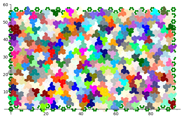
Voici un exemple de construction d'un pavage avec la tuile apériodique. Le calcul est fait dans le logiciel SageMath muni de la version de développement de mon package optionnel slabbe qui peut être installé avec la commande sage -pip install slabbe. Ici, j'utilise le solveur SAT Glucose, développé au LaBRI. On peut installer glucose dans SageMath avec la commande sage -i glucose.
sage: from slabbe.aperiodic_monotile import MonotileSolver
sage: s = MonotileSolver(16, 17)
sage: G = s.draw_one_solution(solver='glucose')
sage: G.save('solution_16x17.png')
sage: G
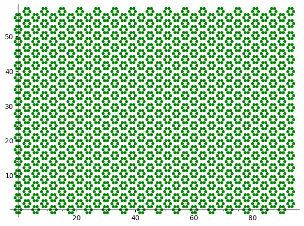
Dans la manière de résoudre la question ci-haut, le problème est représenté par un problème de couverture exacte qui consiste à recouvrir exactement les entiers de 1 à n avec des sous-ensembles choisis dans une liste de sous-ensembles déterminés. Ici, on représente l'espace à recouvrir de manière discrète en comptant 6 points du plan par hexagone (un point pour chaque kite contenu dans un hexagone). Rappelons que la pièce Chapeau qui nous intéresse est formée d'une union d'exactement 8 de ces kites.
sage: s.plot_domain()
Ensuite, on construit une matrice de 0 et de 1 avec autant de colonnes que de points ci-haut (16 * 17 * 2 * 6 = 3264) et autant de lignes qu'il y a de copies isométriques de la pièce intersectant le domaine. Pour chaque copie de la pièce, une ligne dans la matrice contient des 1 exactement dans les colonnes associées aux kites occupés par la pièce.
sage: s.the_dlx_solver()
Dancing links solver for 3264 columns and 7116 rows
Le calcul ci-haut qui a construit la matrice (sparse) indique qu'il y a 7116 copies isométriques de la pièce qui intersectent (complètement ou partiellement) le domaine. Quand on voudra dessiner une solution, on ignorera les pièces incomplètes.
On peut maintenant résoudre le problème.
sage: s = MonotileSolver(8,8)
sage: %time L = s.one_solution()   # l'algo des liens dansants de Knuth est utilisé par défaut
CPU times: user 798 ms, sys: 32.2 ms, total: 830 ms
Wall time: 1min 20s
Le contenu d'une solution est une liste de nombres indiquant les lignes de la matrice de 0/1 à considérer pour former une solution. C'est-à-dire que la sous-matrice restreinte aux lignes données comporte exactement un 1 dans chaque colonne:
sage: L
[81,
 85,
 125,
 128,
 ...
 1772,
 1783,
 1794,
 1815]
Ici, il se trouve que les solveurs SAT sont plus efficaces que l'algo des liens dansants pour trouver une solution:
sage: %time L = s.one_solution(solver='glucose')
CPU times: user 326 ms, sys: 16.1 ms, total: 342 ms
Wall time: 526 ms
sage: %time L = s.one_solution(solver='kissat')
CPU times: user 335 ms, sys: 3.64 ms, total: 339 ms
Wall time: 461 ms
En effet, Glucose se comporte plutôt bien pour résoudre des problèmes de pavages du plan lorsqu'il existe une solution. Mais lorsqu'il n'y a pas de solution, l'algo des liens dansants de Knuth est parfois mieux. Aussi, l'algo des liens dansants de Knuth est très efficace pour énumérer toutes les solutions.
Le solveur Kissat a été ajouté dans SageMath par moi-même comme package optionnel cette année suite à une discussion avec Laurent Simon au café du LaBRI. On peut installer le solveur kissat dans SageMath avec la commande sage -i kissat.
Ici on extrait le contour des pièces d'une solution (tel que chaque arête est dessinée une seule fois afin d'éviter que la découpeuse laser passe deux fois par chaque arête ce qui peut endommager ou brûler le bord des pièces en bois) et on crée un fichier pdf ou svg. Je choisis une taille de 16 double-hexagones horizontalement et 17 verticalement, car cela crée un fichier qui correspond à une taille de 1m x 60cm. C'est la taille de la découpeuse laser à notre disposition:
sage: s = MonotileSolver(16, 17)
sage: tikz = s.one_solution_tikz(solver='glucose')
sage: tikz.pdf('solution_16x17.pdf')
sage: tikz.svg('solution_16x17.svg')     # or
Avec l'aide de David Renault, mon collègue du LaBRI qui enseigne à l'ENSEIRB et qui m'a déjà accompagné dans la réalisation de projets de découpe laser, nous avons découpé le fichier ci-haut le jeudi 27 avril au EirLab, l'atelier de fabrication numérique (FabLab) de l'ENSEIRB-MATMECA:
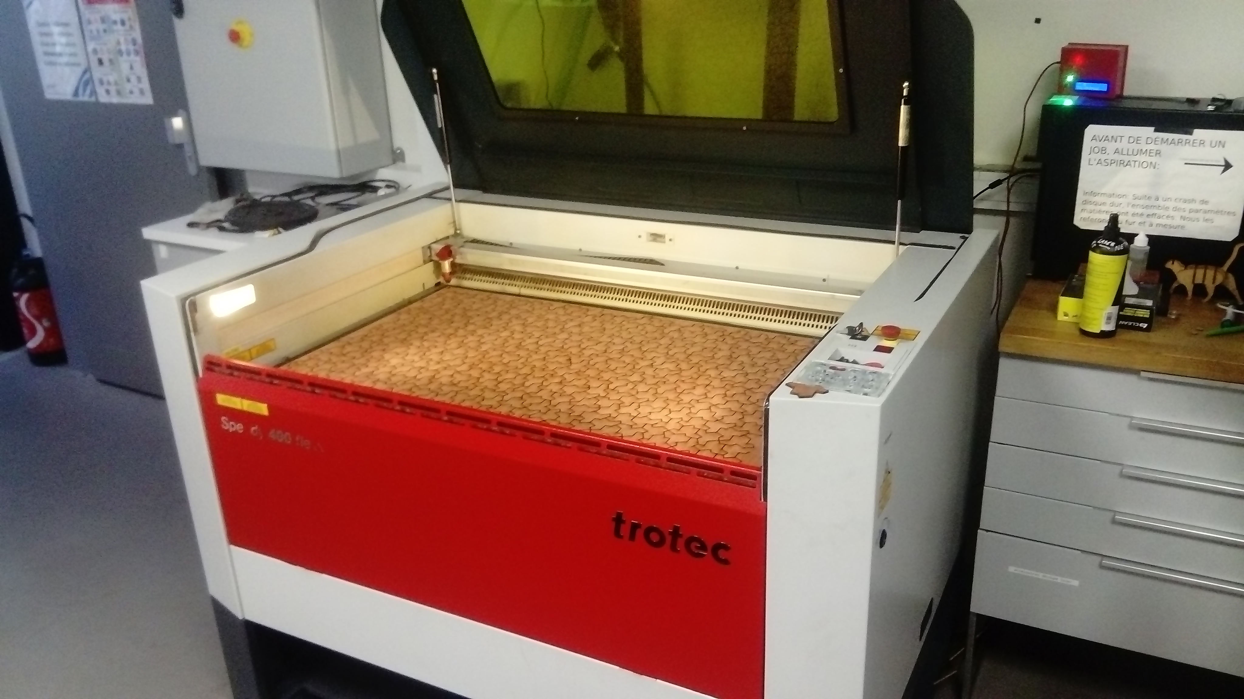
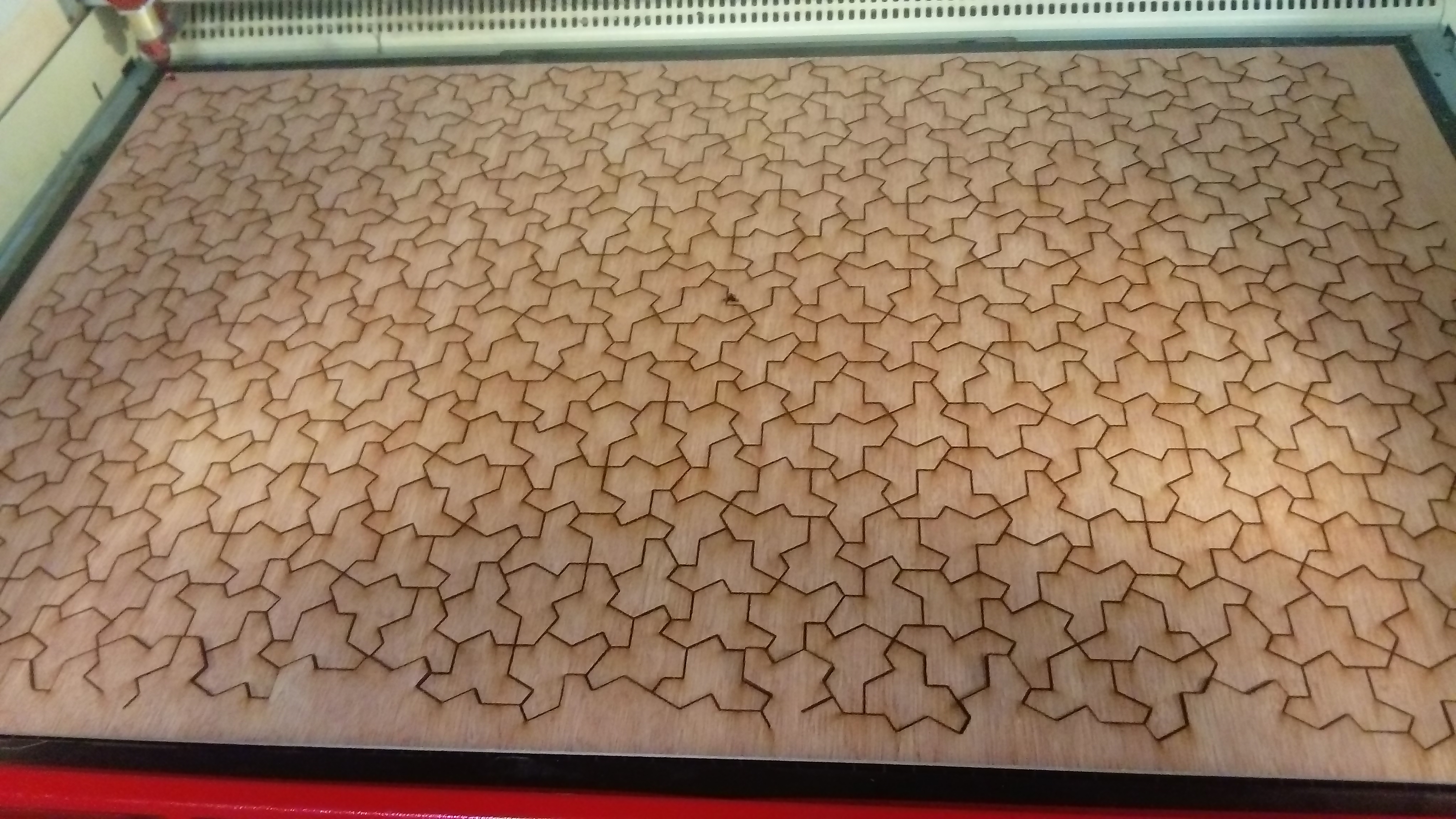
Comme toujours, il faut quelque peu modifier le fichier svg dans Inkscape avant de lancer la découpe laser. Voici le fichier modifié juste avant la découpe.
Maintenant, on peut s'amuser avec les pièces:
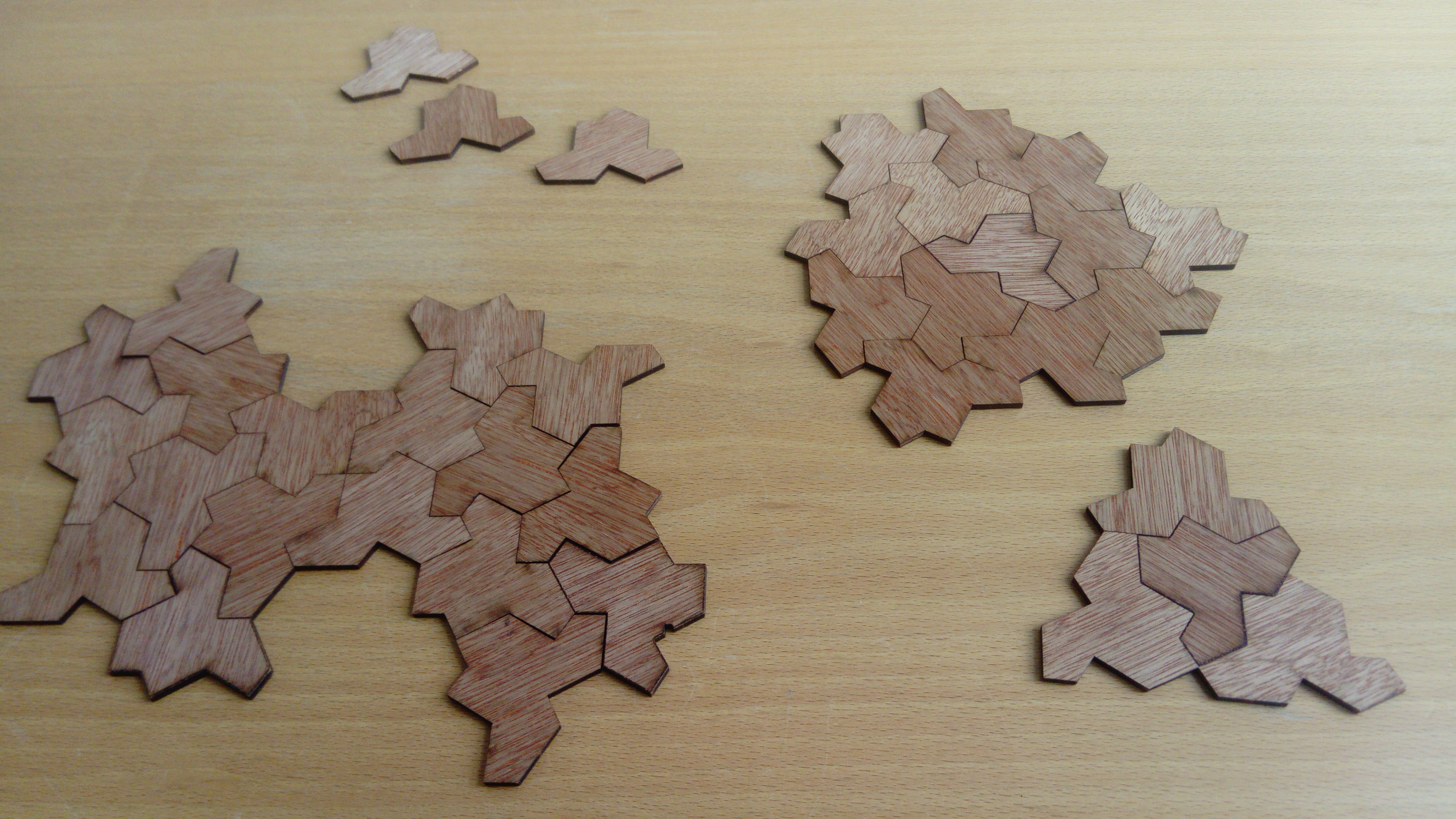
Avec mes garçons, nous avons trouvé une forme intéressante qui recouvre le plan périodiquement à l'exception d'un trou hexagonal. Il se trouve que la même forme peut-être créée de deux façons différentes: sur l'image ci-bas la forme à droite est la globalement la même, mais elle n'est pas obtenue de la même façon que celle en haut à gauche. Pourtant, toutes deux ont le même contour extérieur et le même trou hexagonal.
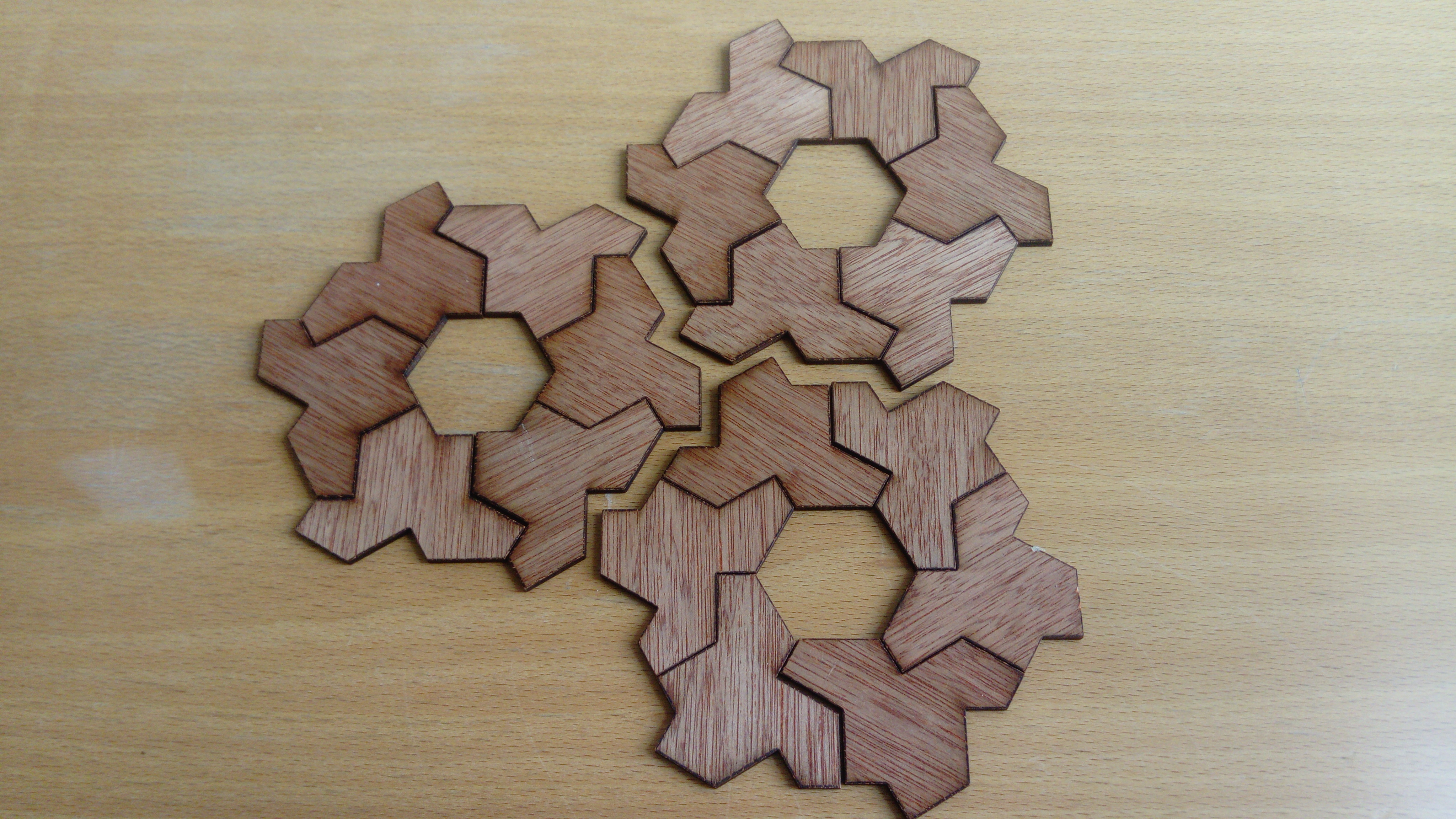
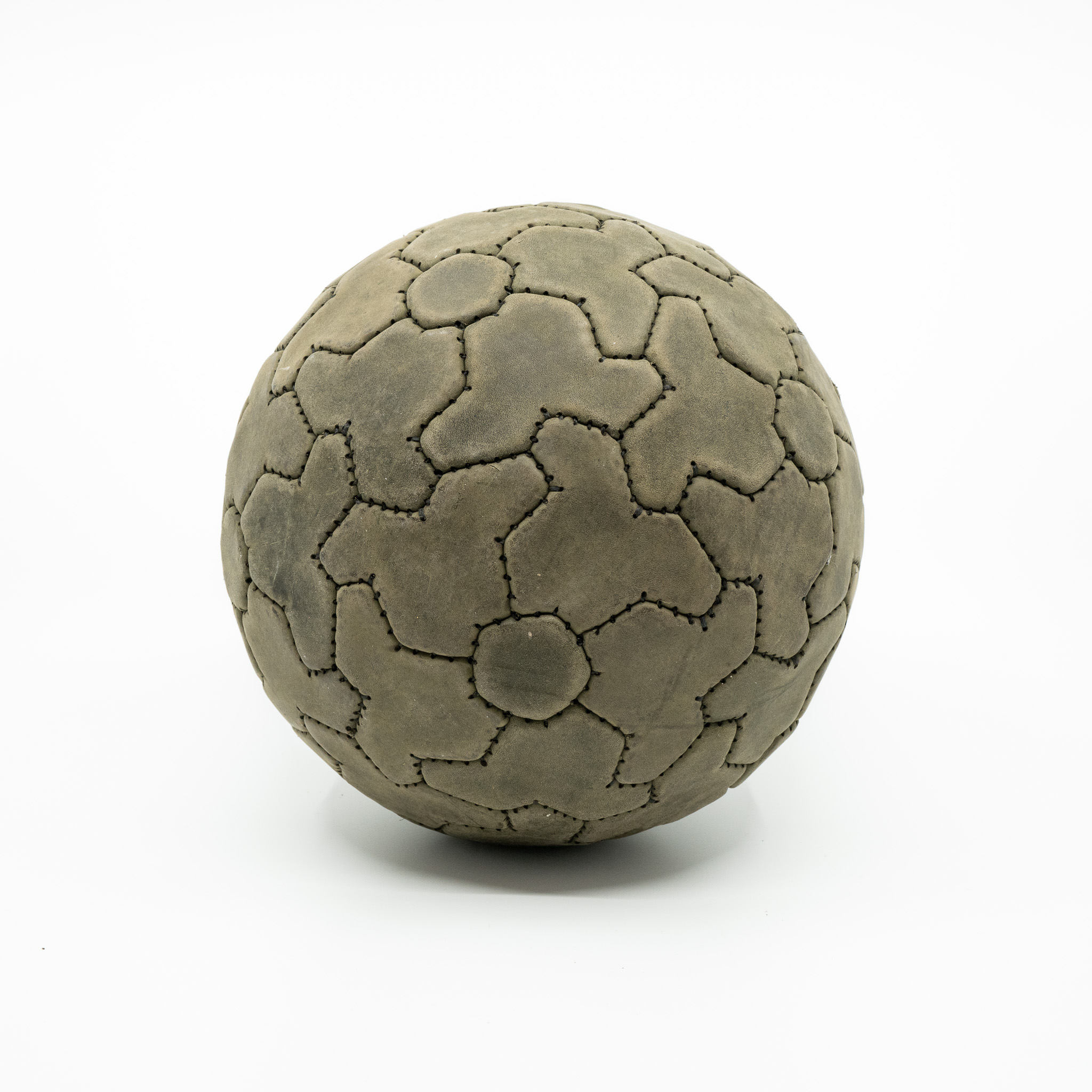
Cette observation, déjà faite par d'autres, a mené au recouvrement d'une sphère avec la pièce et un trou pentagonal:
Un format de tournoi d'ultimate à 7 équipes sur 4 jours dont une seule est qualifiée
28 mars 2023 | Catégories: ultimate | View CommentsDans ce message, je suggère un format de tournoi pour 7 équipes permettant de qualifier une équipe pour l'étape suivante (compétitions nationales par exemple). En bref, la solution suggérée est:
- Faire tournoi à la ronde sur trois jours (2 matchs par jour par équipe)
- Le quatrième jour, les équipes classées #5, #6 et #7 sont éliminées et font un tournoi à la ronde entre elles (donc deux matchs chacune).
- Le quatrième jour, on a les demie-finales #1 vs #4 et #2 vs #3 ainsi que les finales et petite finale.
Plus précisément, voici les détails jour par jour.
Jour 1
Le jour 1, il y a surtout des matchs le top 4 entre eux, et le 5-6-7 entre eux:
| Ronde | Terrain 1 | Terrain 2 |
|---|---|---|
| Ronde 1 | 5 v 6 | 2 v 7 |
| Ronde 2 | 3 v 4 | |
| Ronde 3 | 5 v 7 | 1 v 2 |
| Ronde 4 | 1 v 4 | 3 v 6 |
Note: le match 1v2 peut être devancé de 30 minutes pour laisser plus de temps entre les deux matchs de l'équipe 1.
Jour 2
Le jour 2, il y a des matchs importants pour séparer le top 4 du 5-6-7:
| Ronde | Terrain 1 | Terrain 2 |
|---|---|---|
| Ronde 5 | 2 v 6 | 3 v 7 |
| Ronde 6 | 1 v 5 | |
| Ronde 7 | 2 v 3 | 4 v 6 |
| Ronde 8 | 1 v 7 | 4 v 5 |
Note: le match 4 v 6 peut être devancé de 30 minutes pour laisser plus de temps entre les deux matchs de l'équipe 4.
Jour 3
Le jour 3, il y a surtout des matchs moins importants entre équipes éloignées dans le préclassement:
| Ronde | Terrain 1 | Terrain 2 | Terrain 3 |
|---|---|---|---|
| Ronde 9 | 6 v 7 | ||
| Ronde 10 | 1 v 3 | 2 v 5 | 4 v 7 |
| Ronde 11 | 1 v 6 | 2 v 4 | 3 v 5 |
| Ronde | Terrain 1 | Terrain 2 |
|---|---|---|
| Ronde 9 | 1 v 3 | 6 v 7 |
| Ronde 10 | 2 v 5 | |
| Ronde 11 | 1 v 6 | 4 v 7 |
| Ronde 12 | 2 v 4 | 3 v 5 |
Note: le match 4 v 7 peut être devancé de 30 minutes pour laisser plus de temps entre les deux matchs de l'équipe 4.
Jour 4
- Le jour 4, on fait:
- Tournoi à la ronde entre les équipes #5, #6, #7
- Demi finales: #1 vs #4 et #2 vs #3
- Petite finale
- Finale
Je me suis demandé si à la fin du troisième jour, on fait jouer des pré-demis: #6 vs #3 et #5 vs #4, mais ce n'est pas ce qui est recommandé dans le manuel de USAU Ultimate pour un format à 7 équipes dont une seule est qualifiée pour la montée. En effet, cela donne moins d'importance à bien jouer dans le tournoi à la ronde, et donne moins d'importance aux deux premiers jours. Comme une seule équipe est qualifiée, c'est normal je pense d'en éliminer 3 après le tournoi à la ronde.
Factor complexity of words generated by multidimensional continued fraction algorithms
03 novembre 2022 | Catégories: sage | View CommentsI was asked by email how to compute with SageMath the factor complexity of words generated by multidimensional continued fraction algorithms. I'm copying my answer here so that I can more easily share it.
A) How to calculate the factor complexity of a word
To compute the complexity in factors, we need a finite word and not an infinite infinite word. In the example below, I take a prefix of the Fibonacci word and I compute the number of factors of size 100 and of size 0 to 19:
sage: w = words.FibonacciWord()
sage: w
word: 0100101001001010010100100101001001010010...
sage: prefix = w[:100000]
sage: prefix.number_of_factors(100)
101
sage: [prefix.number_of_factors(i) for i in range(20)]
[1, 2, 3, 4, 5, 6, 7, 8, 9, 10, 11, 12, 13, 14, 15, 16, 17, 18, 19, 20]
The documentation for the number_of_factors method contains more examples, etc.
B) How to construct an S-adic word in SageMath
The method words.s_adic in SageMath allows to construct an S-adic sequence from a directive sequence, a set of substitutions and a sequence of first letters.
For example, we may use Kolakoski word as a directive sequence:
sage: directive_sequence = words.KolakoskiWord()
sage: directive_sequence
word: 1221121221221121122121121221121121221221...
Then, I define the Thue-Morse and Fibonacci substitutions:
sage: tm = WordMorphism('a->ab,b->ba')
sage: fib = WordMorphism('a->ab,b->a')
sage: tm
WordMorphism: a->ab, b->ba
sage: fib
WordMorphism: a->ab, b->a
Then, to define an S-adic sequence, I also need to define the sequence of first letters. Here, it is always the constant sequence a,a,a,a,...:
sage: from itertools import repeat
sage: letters = repeat('a')
I associate the letter 1 in the Kolakoski sequence to the Thue-Morse morphism and 2 to the Fibonacci morphism, this allows to construct an S-adic sequence:
sage: w = words.s_adic(directive_sequence, letters, {1:tm, 2:fib})
sage: w
word: abbaababbaabbaabbaababbaabbaababbaababba...
Then, as above, I can take a prefix and compute its factor complexity:
sage: prefix = w[:100000]
sage: [prefix.number_of_factors(i) for i in range(20)]
[1, 2, 4, 6, 7, 8, 9, 10, 12, 14, 16, 18, 20, 22, 24, 26, 28, 30, 34, 38]
C) Creating an S-adic sequence from Brun algorithm
With the package slabbe, you can construct an S-adic sequence from some of the known Multidimensional Continued Fraction Algorithm.
One can install it by running sage -pip install slabbe in a terminal where sage command exists. Sometimes this does not work.
Then, one may do:
sage: from slabbe.mult_cont_frac import Brun
sage: algo = Brun()
sage: algo
Brun 3-dimensional continued fraction algorithm
sage: D = algo.substitutions()
sage: D
{312: WordMorphism: 1->12, 2->2, 3->3,
 321: WordMorphism: 1->1, 2->21, 3->3,
 213: WordMorphism: 1->13, 2->2, 3->3,
 231: WordMorphism: 1->1, 2->2, 3->31,
 123: WordMorphism: 1->1, 2->23, 3->3,
 132: WordMorphism: 1->1, 2->2, 3->32}
sage: directive_sequence = algo.coding_iterator((1,e,pi))
sage: [next(directive_sequence) for _ in range(10)]
[123, 312, 312, 321, 132, 123, 312, 231, 231, 213]
Construction of the s-adic word from the substitutions and the directive sequence:
sage: from itertools import repeat
sage: D = algo.substitutions()
sage: directive_sequence = algo.coding_iterator((1,e,pi))
sage: words.s_adic(directive_sequence, repeat(1), D)
word: 1232323123233231232332312323123232312323...
Shortcut:
sage: algo.s_adic_word((1,e,pi))
word: 1232323123233231232332312323123232312323...
There are some more examples in the documentation.
This code was used in the creation of the 3-dimensional Continued Fraction Algorithms Cheat Sheets 7 years ago during my postdoc at Université de Liège, Belgium.
Are losers more spirited in ultimate? a data analysis based on 1500 games played during WMUCC, WUCC and CUC 2022
17 octobre 2022 | Mise à jour: 24 octobre 2022 | Catégories: python, ultimate | View CommentsUPDATE (Oct 24, 2022), thanks to comments from reddit: fixed the way standard deviation is presented to avoid misinterpretation, removed the sin(-x) graphics.
When I started to play ultimate in September 2002 in Sherbrooke, the local team Stakatak was just coming back their very first (or maybe second?) participation at the Canadian Ultimate Championship, in the mixed division. I remember they lost all of their nine games and finished 16th out of 16 teams. But they came back in Sherbrooke with the "Spirit of the Game" award which we were very proud of.
What I want to discuss here is not whether the team that lose all its games and wins the Spirit of the Game deserves it or not. The question I want to consider in this blog post is about the evaluation of the spirit of the game in a typical ultimate frisbee game: are we biased by the end result of the game (win vs lose) when we evaluate the opponent's spirit of the game? In particular:
- do we give more spirit points to the opponent team when the opponent has lost against us?
- do we give less spirit points to the opponent team when the opponent has won against us?
The Spirit of the Game
As not everyone reading this post ever played an ultimate frisbee game, let me recall what is the spirit of the game and how it is evaluated nowadays in a tournament. As Ultimate (frisbee) is a self-officiated team sport, the spirit of the game is important. Every team thinks they have a good spirit but not every opponent agree. There are ways for teams to help (or force) them improve their spirit of the game, the most important one being the end of game discussion during which the two teams discuss the game and if necessary any issues that happenned during the game. Another is the evaluation of the spirit of the game by the opponent team, which is made by evaluating 5 subjects:
- Rules Knowledge and Use (4 points)
- Fouls and Body Contact (4 points)
- Fair-Mindedness (4 points)
- Positive Attitude and Self-Control (4 points)
- Communication (4 points)
In Ultimate tournaments, the spirit scores of each team is public and allows to evaluate and rank each team. When a team is low ranked, it shows without ambiguity that the community thinks this team needs to improve because it was badly evaluated by more than one team. This peer-pressure contributes to make teams improve themselve. The ranking is also used to elect a most spirited team which is often given a "Spirit of the game" trophee at the end of the tournament.
Three tournaments considered for the data analysis
For the data analysis, we consider the following three tournaments that were held during Summer 2022:
- World Masters Ultimate Club Championships (WMUCC) 2022, Limerick, Ireland, June 25th to July 2nd 2022
- World Ultimate Club Championships (WUCC) 2022, Cincinnati Ohio, USA, July 23-30, 2022
- Canadian Ultimate Championships (CUC) 2022, Brampton, Ontario, August 18-21, 2022
These tournaments all use the Ultiorganizer website which allows to parse the results with the same Python script which I have made public.
In total, 1540 games were played in these 3 tournaments. Unfortunately, the score or the spirit score was not completed or is not available for all games. Maybe because teams forgot to provide the spirit scores or maybe the game was not played at all. We were able to access all needed data including final score and spirit scores for 1448 of the games (94 %). Since the spirit of both teams gets evaluated during a game, this means 1448 x 2 = 2896 evaluations of a team spirit.
| Tournament | Number of games | Number of games with complete data |
|---|---|---|
| WMUCC 2022 | 589 | 548 (93 %) |
| WUCC 2022 | 652 | 628 (96 %) |
| CUC 2022 | 299 | 272 (91 %) |
| Total | 1540 | 1448 (94 %) |
Average Spirit Points
The average spirit points received by a team is shown in the table below for each of the three considered tournaments.
| Tournament | mean | std |
|---|---|---|
| WMUCC 2022 | 11.307 | 1.830 |
| WUCC 2022 | 10.561 | 1.685 |
| CUC2022 | 10.821 | 2.009 |
Spirit points are on average slightly above 10. Also, at WMUCC, the spirit points were higher in general, slightly above 11. We may interpret this as the fact that older master players playing for a long time were happy to play again at the international level after the pandemia and meet old friends which contributed to have nice spirited games in Limerick (why did not I try to go at Limerick again? I miss my old friends from Epoq or Nsom or Quarantine!).
Average Spirit Points for losers/winners
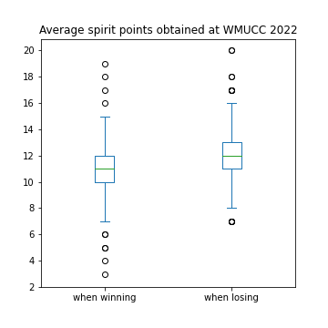
Now let's compare the average spirit points given to the loser of a game vs to the winner of a game. In the three considered tournaments, on average it turns out that the loser of the game always gets more spirit points. See the results in the following table.
| Tournament | When winning (mean; std) | When losing (mean; std) |
|---|---|---|
| WMUCC 2022 | 10.904; 1.756 | 11.709; 1.815 |
| WUCC 2022 | 10.323; 1.707 | 10.800; 1.630 |
| CUC2022 | 10.566; 2.101 | 11.076; 1.882 |
We visualize below the distribution of spirit scores at WMUCC 2022 for losers vs winners with the following box plot graphics made with matplotlib through the pandas library. Small circle indicate what is called flier points. As mentionned in the matplotlib boxplot documentation, "flier points are those past the end of the whiskers".
Are losers more spirited in ultimate?
We can now answer the question asked in the title of this blog post and the answer is yes: the data says that losers are more spirited in Ultimate.
Or, alternatively, we can assume the hypothesis that losers and winners are equally spirited. This assumption implies that players must be biased by the end result of the game when evaluating the opponent's spirit of the game.
Lose-win Bias
It is natural to define the lose-win bias as the difference between the average spirit points obtained by the losing team and the winning team. In other words, how much more spirited are losers than winners? The results is in the following table.
| Tournament | lose-win bias |
|---|---|
| WMUCC 2022 | 0.8043 |
| WUCC 2022 | 0.4768 |
| CUC2022 | 0.5101 |
At WUCC 2022 and CUC 2022, the losing team gets approximatively 0.5 more spirit points than the winning team. During WMUCC 2022, the losing team was obtaining 0.8 more spirit points than the winning team.
Interpretation
How can we interpret these results? Are losers really more spirited or can we accept that we are biased? Is there any other way to interpret the above results?
My interpretation is that we are biased by the end result which means winners and losers will say something like this (if I allow myself to caricature in a provocative way):
"Dear opponent, thanks for losing, we will give you one more spirit point for not making more effort."
"Dear opponent, thanks for the game, you won against us, but your communication was not so good, we give you one point less than we would have usually gave if you would have accepted to lose the game."
Of course I am volontarily exagerating and being a little provocative here to make us think about our own biases. We would never say sentences like this, but, basicaly, I think we might be actually doing this sometimes in a more disguised way.
I think that it is necessary that every ultimate frisbee player know about the existence of this lose-win bias in order to become more objective when evaluating the spirit of the game of the opponent.
Spirit score per score differential
I suggest now to go a bit further in the data analysis. Instead of splitting the spirit points according to the two win or lose cases, we can study the spirit points according to the score differential. This should allow us to answer interesting questions such as:
- Is winning by 1 point the worse thing to do to get a good spirit?
- By how many points should a team win to expect the most spirit points?
- By how many points should a team win to leverage the spirit bias?
Below is a graphics which shows the average spirit point obtained by a team according to the point differential during the three considered tournaments:
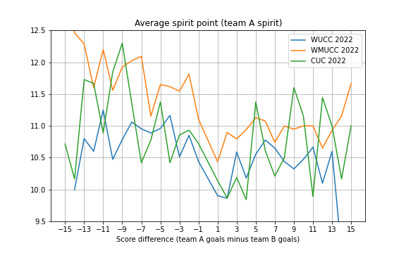
We observe that spirit scores were in general higher at WMUCC 2022. Also, we can see that each curve reach its minimum around +1 or +2, which means you want to win by more than one or two points if you want to win and maximize your spirit points.
Bias per score differential
In what follows, we will discuss the bias per score differential. Here is the graphics summarizing the average lose-win bias according to the end of game point differential (one broken line per tournament):
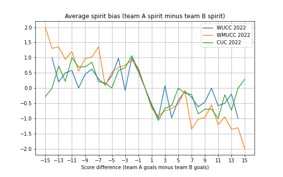
Let's first try to explain the above graphics. The x-axis shows by how much you won the game: +2 means you won the game by 2, and -5 means you lost the game by 5. The graphics shows for each score difference, the average difference between your team spirit score and the opponent spirit score for each of the three tournaments. Take for example the case when your team win by 2, the graphics shows that on average in all of the three tournaments, the spirit score you get is 1 less than the losing team.
Some similarities appear in the three tournaments. On the right part of the graphics, for positive values on the x-axis, the graphic lines are below zero whereas for negative values on the x-axis, the graphic lines are above zero. This essentially means that losers have on average a better spirit evaluation than winners.
One could have expected that winning by one point is worse than winning by two points, because it is in this kind of game that a single action where a travel or fault is called that may affect the outcome of the game, thus affecting the spirit results. But the data shows that winning by 2 is worse than winning by 1 in terms of spirit bias. A possible interpretation goes as follows. When you lose on the universe point, you show to everyone that you were very close to win which is a honorific way of losing. On the other hand, losing by 2 does not allow you to pretend you were close enough to win the game. This may explain why the spirit bias is higher for game finishing by a difference of 2 points compared to 1 point.
Another pattern which is common in each of the three lines is that a local minimum for the lose-win bias is reached when winning by 2. It seems that winning by a higher margin (3, 4, 5 or 6 points) makes the lose-win bias globally closer to zero.
My personnal interpretation is as follows. Winning by 1 or 2 points is not good for your spirit points, because you basically allow your opponent to think that they could have won the game (which may make them biased when evaluating your spirit points). Winning by 5 or 6 points seems to neutralize the win-lose bias. This is enough a point difference which establishes a hierarchy and makes the opponent accept their lost, but not too much that part of the game become meaningless which may impact the fun of both team to play the game.
When the score difference increases, what happens is more chaotic, so I don't know if we can make any safe interpretations, but it seems winning by 7, 8 or 9 is not good for your spirit. And then, winning by exactly 10 points seems also to neutralize the bias. There are fewer games finishing by a difference of more than 10 points, so I will not discuss their statistics here.
Conclusion
To conclude, I would like to recall the real objective of this blog post which is to make the ultimate frisbee players acknowledge the existence of biases when evaluating the opponent's spirit of game, one bias being related to the score result outcome. Once this is acknowledged, the next step is to search for ways to leverage the bias. This task belongs to each and every ultimate frisbee players.
Code and data
I made my code public allows to reproduce the computations and graphics. Everything is in this gitlab repository:
https://gitlab.com/seblabbe/spirit-bias-in-ultimate
The code is written in Python. Data is downloaded with urllib library and stored as csv files. Parsing of Ultiorganizer websites is done in a Python script ultiorganizer_parser.py that I wrote. Analysis of the csv files is done with pandas library with Jupyter notebooks. Graphics are made with matplotlib.
« Previous Page -- Next Page »
Propulsé par Blogofile
S'abonner au Flux RSS
et aux Commentaires.

This work by Sébastien Labbé is licensed under a Creative Commons Attribution-ShareAlike 4.0 International License.