Découpe laser du chapeau, tuile apériodique découverte récemment
25 mai 2023 | Catégories: sage, slabbe spkg, math, découpe laser | View CommentsLe chapeau est une tuile apériodique découverte par David Smith, Joseph Samuel Myers, Craig S. Kaplan, et Chaim Goodman-Strauss le 20 mars 2023. Suite à un exposé donné le 26 mars au National Museum of Mathematics, la nouvelle s'est vite répandue. En effet, cette découverte a été mentionnée les jours suivants dans des blogues puis dans Le New York Times le 28 mars, Le Monde le 29 mars, puis The Guardian et QuantaMagazine le 4 avril. Un vidéo de 20 minutes, réalisé par Passe-Science et publié début le 3 mai, explique le résultat et son contexte.
Déjà des articles proposant des résultats plus approfondis sur la tuile par des experts du domaine sont parus sur arXiv en mai 2023. Ils interprêtent les pavages comme des coupes et projection de réseaux de dimension supérieure. Le deuxième propose même une partition de la fenêtre de l'espace interne, un peu comme pour les pavages de Jeandel-Rao, à la différence qu'ici la partition a des bords fractales ce qui est pour moi une grande surprise.
Comme je faisais une intervention dans l'école de mon garçon à Bègles le 3 mai et au Lycée Kastler de Talence le 4 mai, j'ai réalisé un projet de découpe laser sur la tuile apériodique afin de partager cette récente découverte.
La première question était de construire un pavage d'un rectangle assez grand avec la pièce apériodique. Pour ce faire, j'ai ajouté un nouveau module dans mon package optionel au logiciel SageMath.
Le module réalise une réduction à une instance du problème de la couverture universelle, qui peut être résolu dans SageMath en utilisant l'algorithme des liens dansants de Donald Knuth, les solveurs SAT ou les programmes d'optimisation linéaire (solveur MILP). Le code utilise le système de coordonnées défini dans le fichier validate/kitegrid.pdf qui se trouve dans le code source associé à l'article.
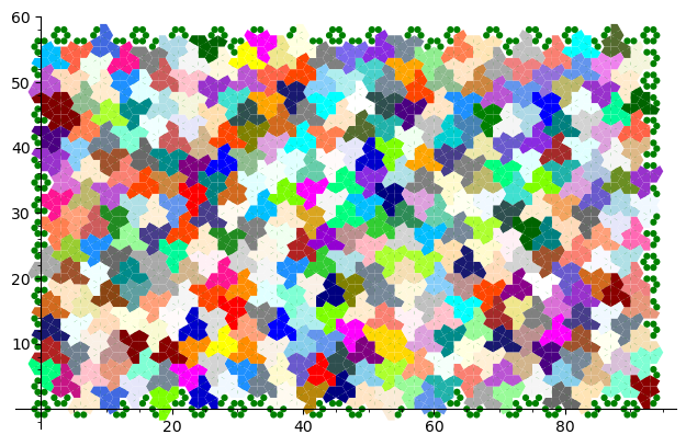
Voici un exemple de construction d'un pavage avec la tuile apériodique. Le calcul est fait dans le logiciel SageMath muni de la version de développement de mon package optionnel slabbe qui peut être installé avec la commande sage -pip install slabbe. Ici, j'utilise le solveur SAT Glucose, développé au LaBRI. On peut installer glucose dans SageMath avec la commande sage -i glucose.
sage: from slabbe.aperiodic_monotile import MonotileSolver
sage: s = MonotileSolver(16, 17)
sage: G = s.draw_one_solution(solver='glucose')
sage: G.save('solution_16x17.png')
sage: G
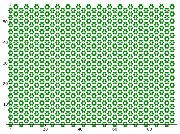
Dans la manière de résoudre la question ci-haut, le problème est représenté par un problème de couverture exacte qui consiste à recouvrir exactement les entiers de 1 à n avec des sous-ensembles choisis dans une liste de sous-ensembles déterminés. Ici, on représente l'espace à recouvrir de manière discrète en comptant 6 points du plan par hexagone (un point pour chaque kite contenu dans un hexagone). Rappelons que la pièce Chapeau qui nous intéresse est formée d'une union d'exactement 8 de ces kites.
sage: s.plot_domain()
Ensuite, on construit une matrice de 0 et de 1 avec autant de colonnes que de points ci-haut (16 * 17 * 2 * 6 = 3264) et autant de lignes qu'il y a de copies isométriques de la pièce intersectant le domaine. Pour chaque copie de la pièce, une ligne dans la matrice contient des 1 exactement dans les colonnes associées aux kites occupés par la pièce.
sage: s.the_dlx_solver()
Dancing links solver for 3264 columns and 7116 rows
Le calcul ci-haut qui a construit la matrice (sparse) indique qu'il y a 7116 copies isométriques de la pièce qui intersectent (complètement ou partiellement) le domaine. Quand on voudra dessiner une solution, on ignorera les pièces incomplètes.
On peut maintenant résoudre le problème.
sage: s = MonotileSolver(8,8)
sage: %time L = s.one_solution()   # l'algo des liens dansants de Knuth est utilisé par défaut
CPU times: user 798 ms, sys: 32.2 ms, total: 830 ms
Wall time: 1min 20s
Le contenu d'une solution est une liste de nombres indiquant les lignes de la matrice de 0/1 à considérer pour former une solution. C'est-à-dire que la sous-matrice restreinte aux lignes données comporte exactement un 1 dans chaque colonne:
sage: L
[81,
 85,
 125,
 128,
 ...
 1772,
 1783,
 1794,
 1815]
Ici, il se trouve que les solveurs SAT sont plus efficaces que l'algo des liens dansants pour trouver une solution:
sage: %time L = s.one_solution(solver='glucose')
CPU times: user 326 ms, sys: 16.1 ms, total: 342 ms
Wall time: 526 ms
sage: %time L = s.one_solution(solver='kissat')
CPU times: user 335 ms, sys: 3.64 ms, total: 339 ms
Wall time: 461 ms
En effet, Glucose se comporte plutôt bien pour résoudre des problèmes de pavages du plan lorsqu'il existe une solution. Mais lorsqu'il n'y a pas de solution, l'algo des liens dansants de Knuth est parfois mieux. Aussi, l'algo des liens dansants de Knuth est très efficace pour énumérer toutes les solutions.
Le solveur Kissat a été ajouté dans SageMath par moi-même comme package optionnel cette année suite à une discussion avec Laurent Simon au café du LaBRI. On peut installer le solveur kissat dans SageMath avec la commande sage -i kissat.
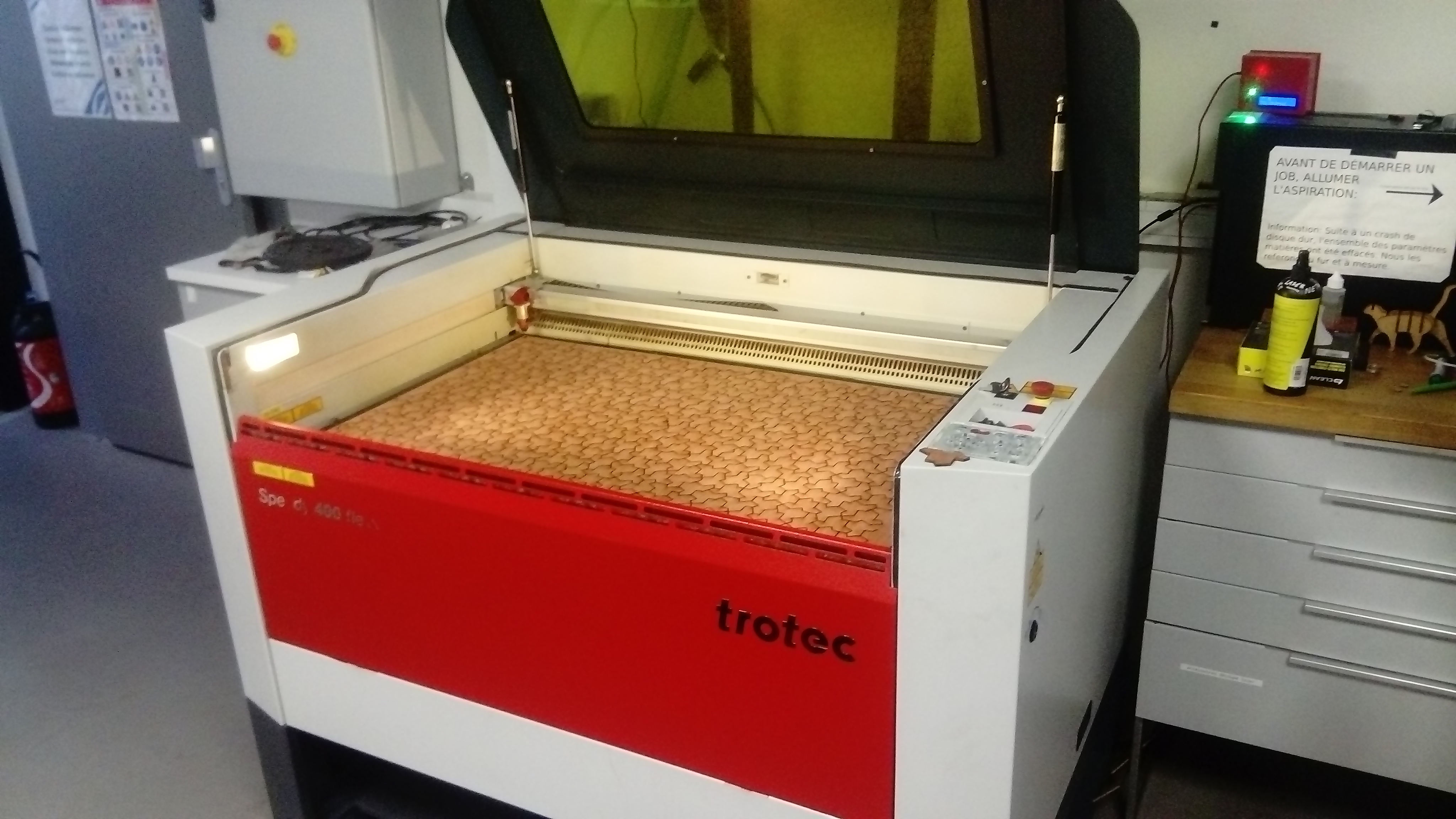
Ici on extrait le contour des pièces d'une solution (tel que chaque arête est dessinée une seule fois afin d'éviter que la découpeuse laser passe deux fois par chaque arête ce qui peut endommager ou brûler le bord des pièces en bois) et on crée un fichier pdf ou svg. Je choisis une taille de 16 double-hexagones horizontalement et 17 verticalement, car cela crée un fichier qui correspond à une taille de 1m x 60cm. C'est la taille de la découpeuse laser à notre disposition:
sage: s = MonotileSolver(16, 17)
sage: tikz = s.one_solution_tikz(solver='glucose')
sage: tikz.pdf('solution_16x17.pdf')
sage: tikz.svg('solution_16x17.svg')     # or
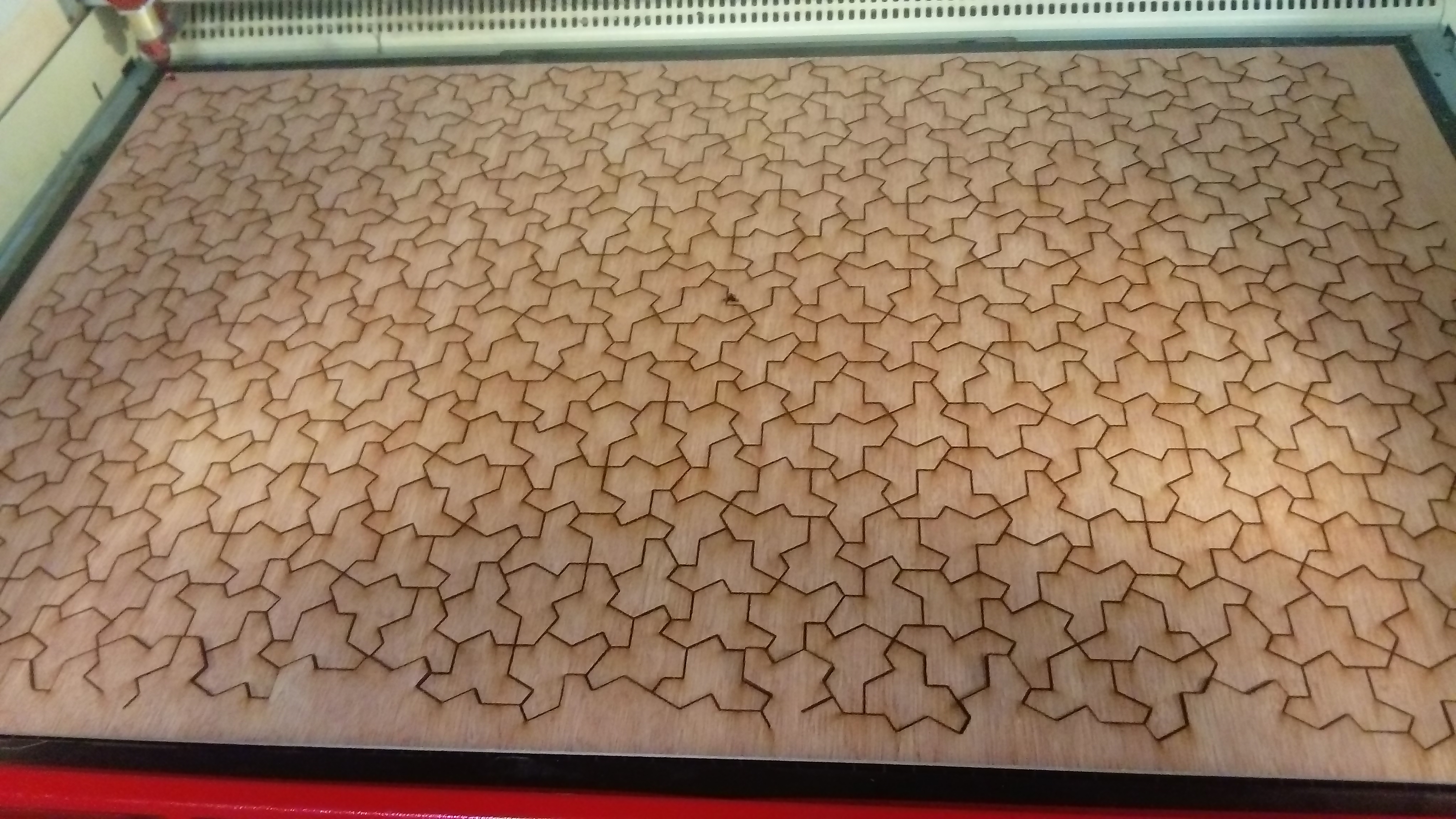
Avec l'aide de David Renault, mon collègue du LaBRI qui enseigne à l'ENSEIRB et qui m'a déjà accompagné dans la réalisation de projets de découpe laser, nous avons découpé le fichier ci-haut le jeudi 27 avril au EirLab, l'atelier de fabrication numérique (FabLab) de l'ENSEIRB-MATMECA:
Comme toujours, il faut quelque peu modifier le fichier svg dans Inkscape avant de lancer la découpe laser. Voici le fichier modifié juste avant la découpe.
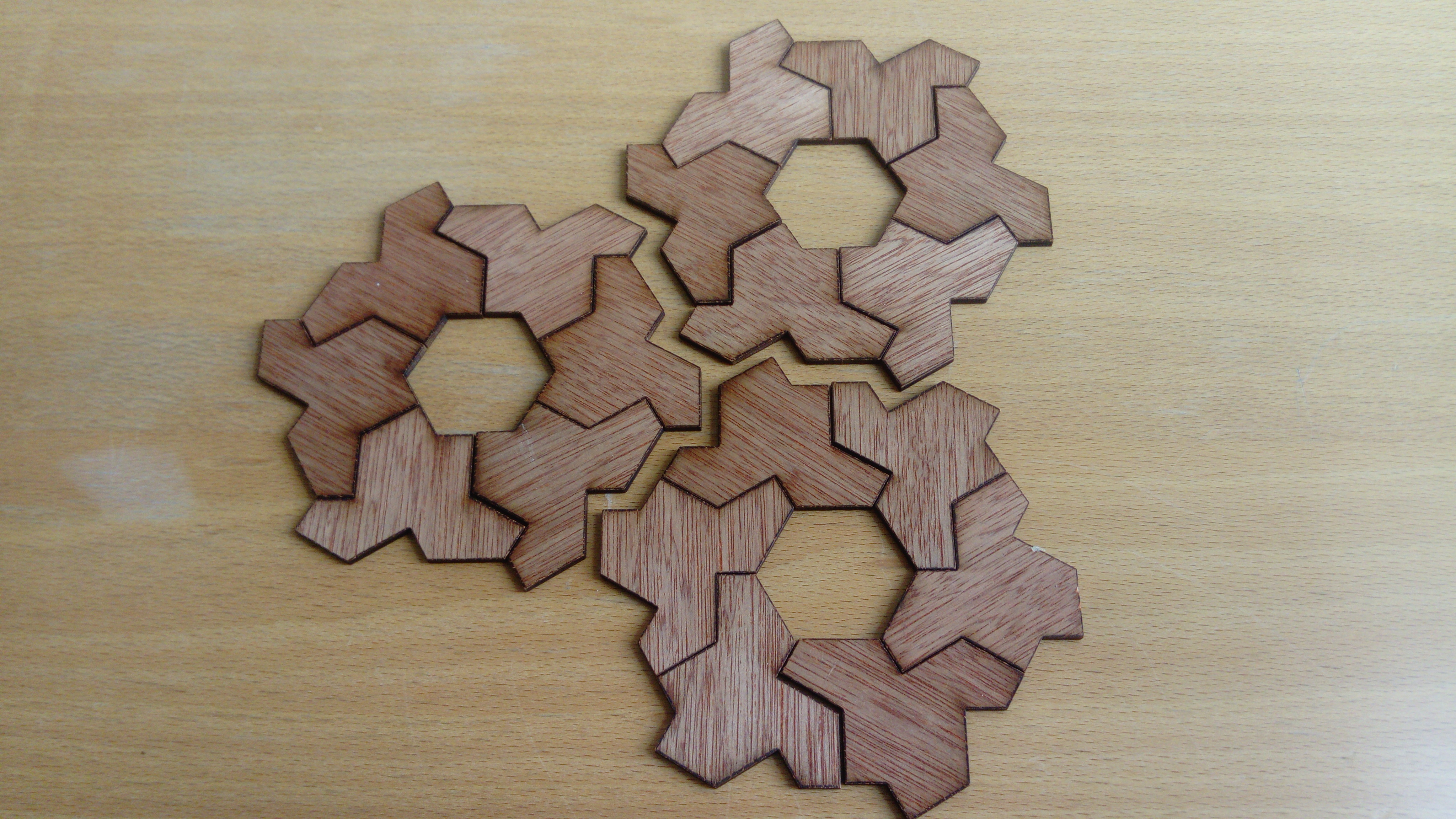
Maintenant, on peut s'amuser avec les pièces:
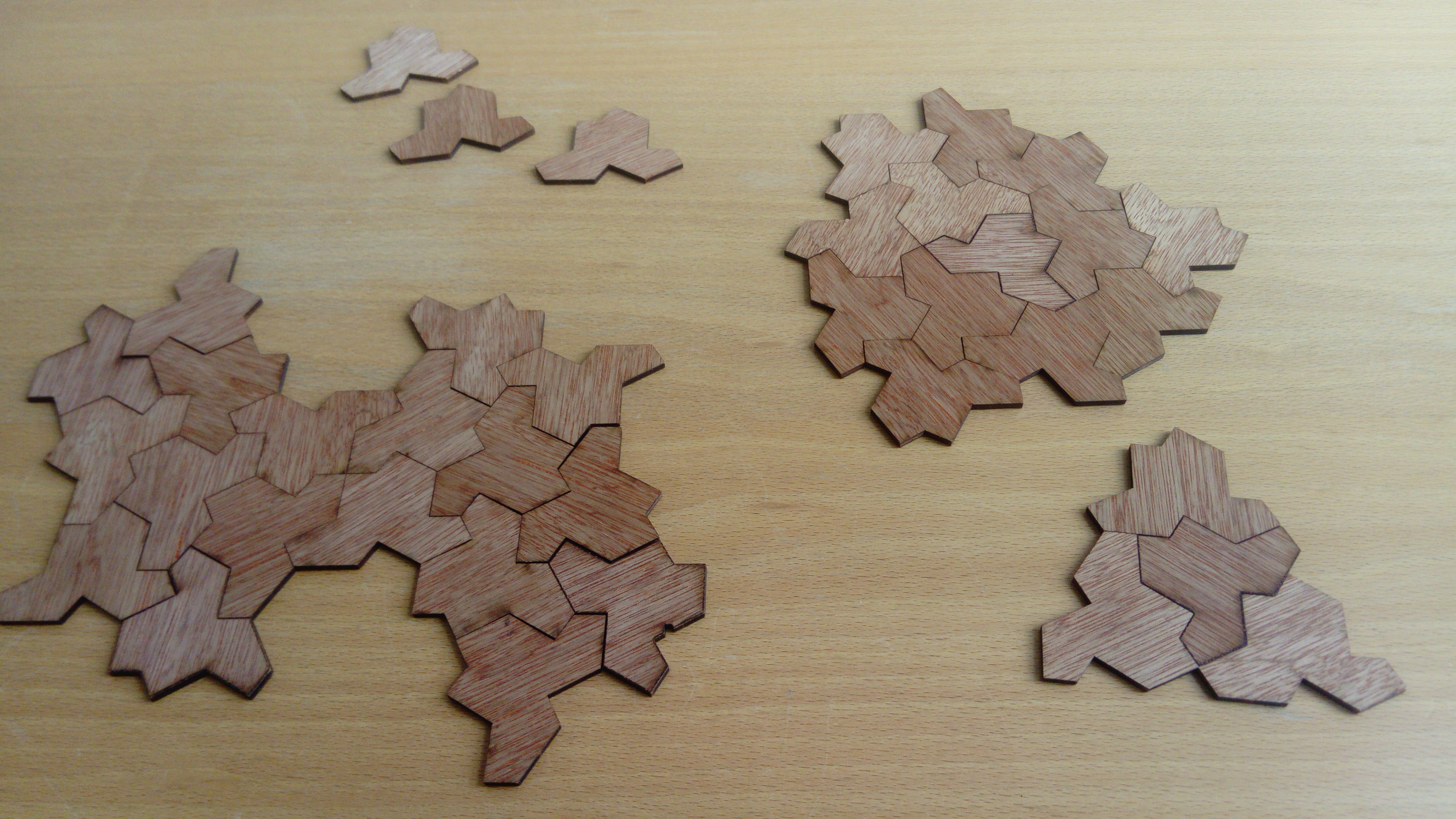
Avec mes garçons, nous avons trouvé une forme intéressante qui recouvre le plan périodiquement à l'exception d'un trou hexagonal. Il se trouve que la même forme peut-être créée de deux façons différentes: sur l'image ci-bas la forme à droite est la globalement la même, mais elle n'est pas obtenue de la même façon que celle en haut à gauche. Pourtant, toutes deux ont le même contour extérieur et le même trou hexagonal.
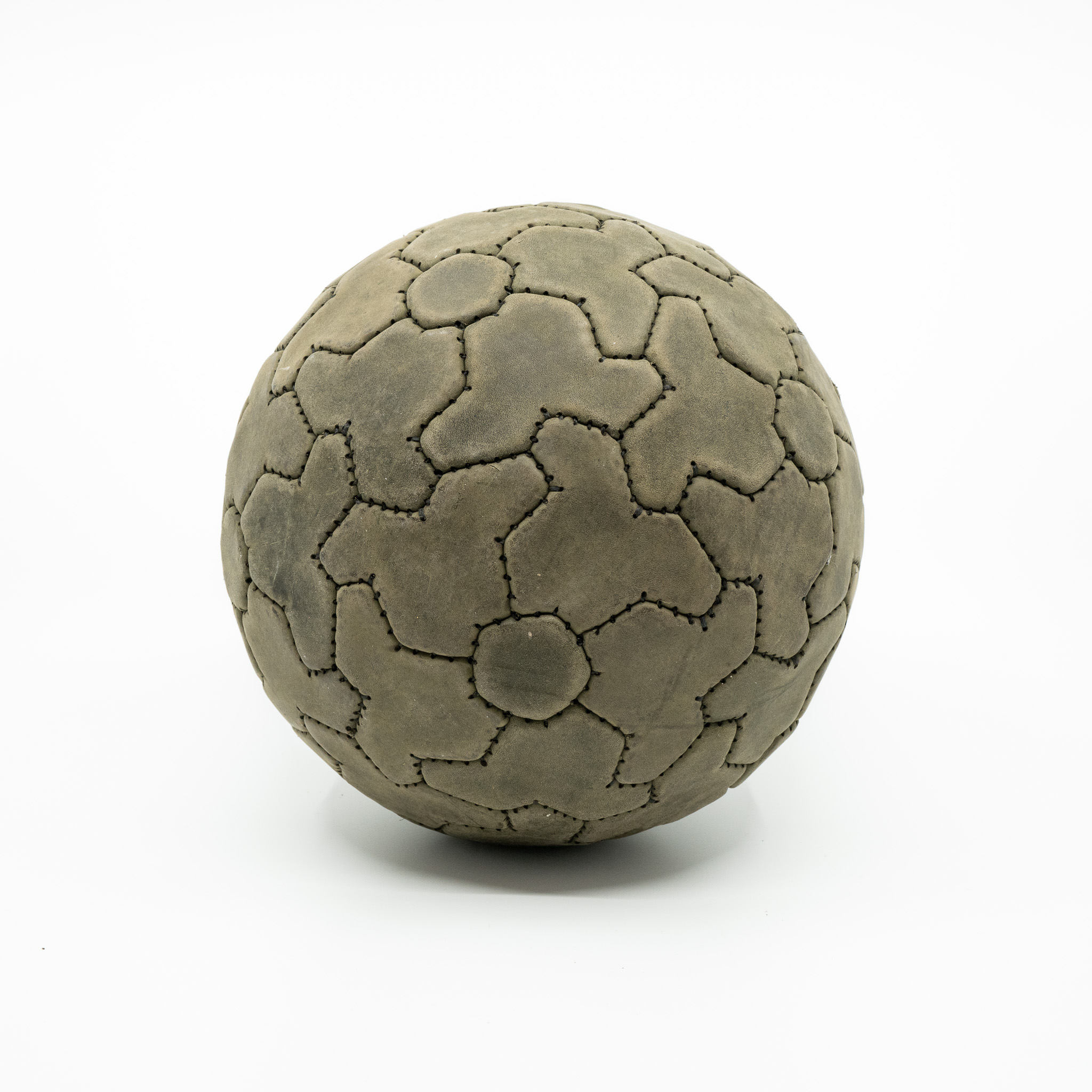
Cette observation, déjà faite par d'autres, a mené au recouvrement d'une sphère avec la pièce et un trou pentagonal:
Computer experiments for the Lyapunov exponent for MCF algorithms when dimension is larger than 3
27 mars 2020 | Catégories: sage, slabbe spkg, math | View CommentsIn November 2015, I wanted to share intuitions I developped on the behavior of various distinct Multidimensional Continued Fractions algorithms obtained from various kind of experiments performed with them often involving combinatorics and digitial geometry but also including the computation of their first two Lyapunov exponents.
As continued fractions are deeply related to the combinatorics of Sturmian sequences which can be seen as the digitalization of a straight line in the grid \(\mathbb{Z}^2\), the multidimensional continued fractions algorithm are related to the digitalization of a straight line and hyperplanes in \(\mathbb{Z}^d\).
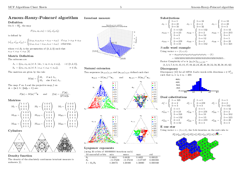
This is why I shared those experiments in what I called 3-dimensional Continued Fraction Algorithms Cheat Sheets because of its format inspired from typical cheat sheets found on the web. All of the experiments can be reproduced using the optional SageMath package slabbe where I share my research code. People asked me whether I was going to try to publish those Cheat Sheets, but I was afraid the format would change the organization of the information and data in each page, so, in the end, I never submitted those Cheat Sheets anywhere.
Here I should say that \(d\) stands for the dimension of the vector space on which the involved matrices act and \(d-1\) is the dimension of the projective space on which the algorithm acts.
One of the consequence of the Cheat Sheets is that it made us realize that the algorithm proposed by Julien Cassaigne had the same first two Lyapunov exponents as the Selmer algorithm (first 3 significant digits were the same). Julien then discovered the explanation as its algorithm is conjugated to some semi-sorted version of the Selmer algorihm. This result was shared during WORDS 2017 conference. Julien Leroy, Julien Cassaigne and I are still working on the extended version of the paper. It is taking longer mainly because of my fault because I have been working hard on aperiodic Wang tilings in the previous 2 years.
During July 2019, Wolfgang, Valérie and Jörg asked me to perform computations of the first two Lyapunov exponents for \(d\)-dimensional Multidimensional Continued Fraction algorithms for \(d\) larger than 3. The main question of interest is whether the second Lyapunov exponent keeps being negative as the dimension increases. This property is related to the notion of strong convergence almost everywhere of the simultaneous diopantine approximations provided by the algorithm of a fixed vector of real numbers. It did not take me too long to update my package since I had started to generalize my code to larger dimensions during Fall 2017. It turns out that, as the dimension increases, all known MCF algorithms have their second Lyapunov exponent become positive. My computations were thus confirming what they eventually published in their preprint in November 2019.
My motivation for sharing the results is the conference Multidimensional Continued Fractions and Euclidean Dynamics held this week (supposed to be held in Lorentz Center, March 23-27 2020, it got cancelled because of the corona virus) where some discussions during video meetings are related to this subject.
The computations performed below can be summarized in one graphics showing the values of \(1-\theta_2/\theta_1\) with respect to \(d\) for various \(d\)-dimensional MCF algorithms. It seems that \(\theta_2\) is negative up to dimension 10 for Brun, up to dimension 4 for Selmer and up to dimension 5 for ARP.
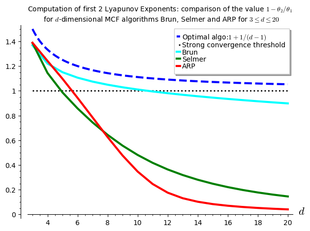
I have to say that I was disapointed by the results because the algorithm Arnoux-Rauzy-Poincaré (ARP) that Valérie and I introduced was not performing so well as its second Lyapunov exponent seems to become positive for dimension \(d\geq 6\). I had good expectations for ARP because it reaches the highest value for \(1-\theta_2/\theta_1\) in the computations performed in the Cheat Sheets, thus better than Brun, better than Selmer when \(d=3\).
The algorithm for the computation of the first two Lyapunov exponents was provided to me by Vincent Delecroix. It applies the algorithm \((v,w)\mapsto(M^{-1}v,M^T w)\) millions of times. The evolution of the size of the vector \(v\) gives the first Lyapunov exponent. The evolution of the size of the vector \(w\) gives the second Lyapunov exponent. Since the computation is performed on 64-bits double floating point number, their are numerical issues to deal with. This is why some Gramm Shimdts operation is performed on the vector \(w\) at each time the vectors are renormalized to keep the vector \(w\) orthogonal to \(v\). Otherwise, the numerical errors cumulate and the computed value for the \(\theta_2\) becomes the same as \(\theta_1\). You can look at the algorithm online starting at line 1723 of the file mult_cont_frac_pyx.pyx from my optional package.
I do not know from where Vincent took that algorithm. So, I do not know how exact it is and whether there exits any proof of lower bounds and upper bounds on the computations being performed. What I can say is that it is quite reliable in the sense that is returns the same values over and over again (by that I mean 3 common most significant digits) with any fixed inputs (number of iterations).
Below, I show the code illustrating how to reproduce the results.
The version 0.6 (November 2019) of my package slabbe includes the necessary code to deal with some \(d\)-dimensional Multidimensional Continued Fraction (MCF) algorithms. Its documentation is available online. It is a PIP package, so it can be installed like this:
sage -pip install slabbe
Recall that the dimension \(d\) below is the linear one and \(d-1\) is the dimension of the space for the corresponding projective algorithm.
Import the Brun, Selmer and Arnoux-Rauzy-Poincaré MCF algorithms from the optional package:
sage: from slabbe.mult_cont_frac import Brun, Selmer, ARP
The computation of the first two Lyapunov exponents performed on one single orbit:
sage: Brun(dim=3).lyapunov_exponents(n_iterations=10^7)
(0.30473782969922547, -0.11220958022368056, 1.3682167728713919)
The starting point is taken randomly, but the results of the form of a 3-tuple \((\theta_1,\theta_2,1-\theta_2/\theta_1)\) are about the same:
sage: Brun(dim=3).lyapunov_exponents(n_iterations=10^7)
(0.30345018206132324, -0.11171509867725296, 1.3681497170915415)
Increasing the dimension \(d\) yields:
sage: Brun(dim=4).lyapunov_exponents(n_iterations=10^7)
(0.32639514522732005, -0.07191456560115839, 1.2203297648654456)
sage: Brun(dim=5).lyapunov_exponents(n_iterations=10^7)
(0.30918877340506756, -0.0463930802132972, 1.1500477514185734)
It performs an orbit of length \(10^7\) in about .5 seconds, of length \(10^8\) in about 5 seconds and of length \(10^9\) in about 50 seconds:
sage: %time Brun(dim=3).lyapunov_exponents(n_iterations=10^7)
CPU times: user 540 ms, sys: 0 ns, total: 540 ms
Wall time: 539 ms
(0.30488799356325225, -0.11234354880132114, 1.3684748208296182)
sage: %time Brun(dim=3).lyapunov_exponents(n_iterations=10^8)
CPU times: user 5.09 s, sys: 0 ns, total: 5.09 s
Wall time: 5.08 s
(0.30455473631148755, -0.11217550411862384, 1.3683262505689446)
sage: %time Brun(dim=3).lyapunov_exponents(n_iterations=10^9)
CPU times: user 51.2 s, sys: 0 ns, total: 51.2 s
Wall time: 51.2 s
(0.30438755982577026, -0.11211562816821799, 1.368331834035505)
Here, in what follows, I must admit that I needed to do a small fix to my package, so the code below will not work in version 0.6 of my package, I will update my package in the next days in order that the computations below can be reproduced:
sage: from slabbe.lyapunov import lyapunov_comparison_table
For each \(3\leq d\leq 20\), I compute 30 orbits and I show the most significant digits and the standard deviation of the 30 values computed.
For Brun algorithm:
sage: algos = [Brun(d) for d in range(3,21)]
sage: %time lyapunov_comparison_table(algos, n_orbits=30, n_iterations=10^7, ncpus=8)
CPU times: user 190 ms, sys: 2.8 s, total: 2.99 s
Wall time: 6min 31s
  Algorithm     \#Orbits   $\theta_1$ (std)     $\theta_2$ (std)      $1-\theta_2/\theta_1$ (std)
+-------------+----------+--------------------+---------------------+-----------------------------+
  Brun (d=3)    30         0.3045 (0.00040)     -0.1122 (0.00017)     1.3683 (0.00022)
  Brun (d=4)    30         0.32632 (0.000055)   -0.07188 (0.000051)   1.2203 (0.00014)
  Brun (d=5)    30         0.30919 (0.000032)   -0.04647 (0.000041)   1.1503 (0.00013)
  Brun (d=6)    30         0.28626 (0.000027)   -0.03043 (0.000035)   1.1063 (0.00012)
  Brun (d=7)    30         0.26441 (0.000024)   -0.01966 (0.000027)   1.0743 (0.00010)
  Brun (d=8)    30         0.24504 (0.000027)   -0.01207 (0.000024)   1.04926 (0.000096)
  Brun (d=9)    30         0.22824 (0.000021)   -0.00649 (0.000026)   1.0284 (0.00012)
  Brun (d=10)   30         0.2138 (0.00098)     -0.0022 (0.00015)     1.0104 (0.00074)
  Brun (d=11)   30         0.20085 (0.000015)   0.00106 (0.000022)    0.9947 (0.00011)
  Brun (d=12)   30         0.18962 (0.000017)   0.00368 (0.000021)    0.9806 (0.00011)
  Brun (d=13)   30         0.17967 (0.000011)   0.00580 (0.000020)    0.9677 (0.00011)
  Brun (d=14)   30         0.17077 (0.000011)   0.00755 (0.000021)    0.9558 (0.00012)
  Brun (d=15)   30         0.16278 (0.000012)   0.00900 (0.000017)    0.9447 (0.00010)
  Brun (d=16)   30         0.15556 (0.000011)   0.01022 (0.000013)    0.93433 (0.000086)
  Brun (d=17)   30         0.149002 (9.5e-6)    0.01124 (0.000015)    0.9246 (0.00010)
  Brun (d=18)   30         0.14303 (0.000010)   0.01211 (0.000019)    0.9153 (0.00014)
  Brun (d=19)   30         0.13755 (0.000012)   0.01285 (0.000018)    0.9065 (0.00013)
  Brun (d=20)   30         0.13251 (0.000011)   0.01349 (0.000019)    0.8982 (0.00014)
For Selmer algorithm:
sage: algos = [Selmer(d) for d in range(3,21)]
sage: %time lyapunov_comparison_table(algos, n_orbits=30, n_iterations=10^7, ncpus=8)
CPU times: user 203 ms, sys: 2.78 s, total: 2.98 s
Wall time: 6min 27s
  Algorithm       \#Orbits   $\theta_1$ (std)     $\theta_2$ (std)      $1-\theta_2/\theta_1$ (std)
+---------------+----------+--------------------+---------------------+-----------------------------+
  Selmer (d=3)    30         0.1827 (0.00041)     -0.0707 (0.00017)     1.3871 (0.00029)
  Selmer (d=4)    30         0.15808 (0.000058)   -0.02282 (0.000036)   1.1444 (0.00023)
  Selmer (d=5)    30         0.13199 (0.000033)   0.00176 (0.000034)    0.9866 (0.00026)
  Selmer (d=6)    30         0.11205 (0.000017)   0.01595 (0.000036)    0.8577 (0.00031)
  Selmer (d=7)    30         0.09697 (0.000012)   0.02481 (0.000030)    0.7442 (0.00032)
  Selmer (d=8)    30         0.085340 (8.5e-6)    0.03041 (0.000032)    0.6437 (0.00036)
  Selmer (d=9)    30         0.076136 (5.9e-6)    0.03379 (0.000032)    0.5561 (0.00041)
  Selmer (d=10)   30         0.068690 (5.5e-6)    0.03565 (0.000023)    0.4810 (0.00032)
  Selmer (d=11)   30         0.062557 (4.4e-6)    0.03646 (0.000021)    0.4172 (0.00031)
  Selmer (d=12)   30         0.057417 (3.6e-6)    0.03654 (0.000017)    0.3636 (0.00028)
  Selmer (d=13)   30         0.05305 (0.000011)   0.03615 (0.000018)    0.3186 (0.00032)
  Selmer (d=14)   30         0.04928 (0.000060)   0.03546 (0.000051)    0.2804 (0.00040)
  Selmer (d=15)   30         0.046040 (2.0e-6)    0.03462 (0.000013)    0.2482 (0.00027)
  Selmer (d=16)   30         0.04318 (0.000011)   0.03365 (0.000014)    0.2208 (0.00028)
  Selmer (d=17)   30         0.040658 (3.3e-6)    0.03263 (0.000013)    0.1974 (0.00030)
  Selmer (d=18)   30         0.038411 (2.7e-6)    0.031596 (9.8e-6)     0.1774 (0.00022)
  Selmer (d=19)   30         0.036399 (2.2e-6)    0.030571 (8.0e-6)     0.1601 (0.00019)
  Selmer (d=20)   30         0.0346 (0.00011)     0.02955 (0.000093)    0.1452 (0.00019)
For Arnoux-Rauzy-Poincaré algorithm:
sage: algos = [ARP(d) for d in range(3,21)]
sage: %time lyapunov_comparison_table(algos, n_orbits=30, n_iterations=10^7, ncpus=8)
CPU times: user 226 ms, sys: 2.76 s, total: 2.99 s
Wall time: 13min 20s
  Algorithm                        \#Orbits   $\theta_1$ (std)     $\theta_2$ (std)      $1-\theta_2/\theta_1$ (std)
+--------------------------------+----------+--------------------+---------------------+-----------------------------+
  Arnoux-Rauzy-Poincar\'e (d=3)    30         0.4428 (0.00056)     -0.1722 (0.00025)     1.3888 (0.00016)
  Arnoux-Rauzy-Poincar\'e (d=4)    30         0.6811 (0.00020)     -0.16480 (0.000085)   1.24198 (0.000093)
  Arnoux-Rauzy-Poincar\'e (d=5)    30         0.7982 (0.00012)     -0.0776 (0.00010)     1.0972 (0.00013)
  Arnoux-Rauzy-Poincar\'e (d=6)    30         0.83563 (0.000091)   0.0475 (0.00010)      0.9432 (0.00012)
  Arnoux-Rauzy-Poincar\'e (d=7)    30         0.8363 (0.00011)     0.1802 (0.00016)      0.7845 (0.00020)
  Arnoux-Rauzy-Poincar\'e (d=8)    30         0.8213 (0.00013)     0.3074 (0.00023)      0.6257 (0.00028)
  Arnoux-Rauzy-Poincar\'e (d=9)    30         0.8030 (0.00012)     0.4205 (0.00017)      0.4763 (0.00022)
  Arnoux-Rauzy-Poincar\'e (d=10)   30         0.7899 (0.00011)     0.5160 (0.00016)      0.3467 (0.00020)
  Arnoux-Rauzy-Poincar\'e (d=11)   30         0.7856 (0.00014)     0.5924 (0.00020)      0.2459 (0.00022)
  Arnoux-Rauzy-Poincar\'e (d=12)   30         0.7883 (0.00010)     0.6497 (0.00012)      0.1759 (0.00014)
  Arnoux-Rauzy-Poincar\'e (d=13)   30         0.7930 (0.00010)     0.6892 (0.00014)      0.1309 (0.00014)
  Arnoux-Rauzy-Poincar\'e (d=14)   30         0.7962 (0.00012)     0.7147 (0.00015)      0.10239 (0.000077)
  Arnoux-Rauzy-Poincar\'e (d=15)   30         0.7974 (0.00012)     0.7309 (0.00014)      0.08340 (0.000074)
  Arnoux-Rauzy-Poincar\'e (d=16)   30         0.7969 (0.00015)     0.7411 (0.00014)      0.07010 (0.000048)
  Arnoux-Rauzy-Poincar\'e (d=17)   30         0.7960 (0.00014)     0.7482 (0.00014)      0.06005 (0.000050)
  Arnoux-Rauzy-Poincar\'e (d=18)   30         0.7952 (0.00013)     0.7537 (0.00014)      0.05218 (0.000046)
  Arnoux-Rauzy-Poincar\'e (d=19)   30         0.7949 (0.00012)     0.7584 (0.00013)      0.04582 (0.000035)
  Arnoux-Rauzy-Poincar\'e (d=20)   30         0.7948 (0.00014)     0.7626 (0.00013)      0.04058 (0.000025)
The computation of the figure shown above is done with the code below:
sage: brun_list = [1.3683, 1.2203, 1.1503, 1.1063, 1.0743, 1.04926, 1.0284, 1.0104, 0.9947, 0.9806, 0.9677, 0.9558, 0.9447, 0.93433, 0.9246, 0.9153, 0.9065, 0.8982]
sage: selmer_list = [ 1.3871, 1.1444, 0.9866, 0.8577, 0.7442, 0.6437, 0.5561, 0.4810, 0.4172, 0.3636, 0.3186, 0.2804, 0.2482, 0.2208, 0.1974, 0.1774, 0.1601, 0.1452]
sage: arp_list = [1.3888, 1.24198, 1.0972, 0.9432, 0.7845, 0.6257, 0.4763, 0.3467, 0.2459, 0.1759, 0.1309, 0.10239, 0.08340, 0.07010, 0.06005, 0.05218, 0.04582, 0.04058]
sage: brun_points = list(enumerate(brun_list, start=3))
sage: selmer_points = list(enumerate(selmer_list, start=3))
sage: arp_points = list(enumerate(arp_list, start=3))
sage: G = Graphics()
sage: G += plot(1+1/(x-1), x, 3, 20, legend_label='Optimal algo:$1+1/(d-1)$', linestyle='dashed', color='blue', thickness=3)
sage: G += line([(3,1), (20,1)], color='black', legend_label='Strong convergence threshold', linestyle='dotted', thickness=2)
sage: G += line(brun_points, legend_label='Brun', color='cyan', thickness=3)
sage: G += line(selmer_points, legend_label='Selmer', color='green', thickness=3)
sage: G += line(arp_points, legend_label='ARP', color='red', thickness=3)
sage: G.ymin(0)
sage: G.axes_labels(['$d$',''])
sage: G.show(title='Computation of first 2 Lyapunov Exponents: comparison of the value $1-\\theta_2/\\theta_1$\n for $d$-dimensional MCF algorithms Brun, Selmer and ARP for $3\\leq d\\leq 20$')
Comparison of Wang tiling solvers
12 décembre 2018 | Catégories: sage, slabbe spkg, math | View CommentsDuring the last year, I have written a Python module to deal with Wang tiles containing about 4K lines of code including doctests and documentation.
It can be installed like this:
sage -pip install slabbe
It can be used like this:
sage: from slabbe import WangTileSet
sage: tiles = [(2,4,2,1), (2,2,2,0), (1,1,3,1), (1,2,3,2), (3,1,3,3),
....: (0,1,3,1), (0,0,0,1), (3,1,0,2), (0,2,1,2), (1,2,1,4), (3,3,1,2)]
sage: T0 = WangTileSet([tuple(str(a) for a in t) for t in tiles])
sage: T0.tikz(ncolumns=11).pdf()
The module on wang tiles contains a class WangTileSolver which contains three reductions of the Wang tiling problem the first using MILP solvers, the second using SAT solvers and the third using Knuth's dancing links.
Here is one example of a tiling found using the dancing links reduction:
sage: %time tiling = T0.solver(10,10).solve(solver='dancing_links')
CPU times: user 36 ms, sys: 12 ms, total: 48 ms
Wall time: 65.5 ms
sage: tiling.tikz().pdf()
All these reductions now allow me to compare the efficiency of various types of solvers restricted to the Wang tiling type of problems. Here is the list of solvers that I often use.
| Solver | Description |
|---|---|
| 'Gurobi' | MILP solver |
| 'GLPK' | MILP solver |
| 'PPL' | MILP solver |
| 'LP' | a SAT solver using a reduction to LP |
| 'cryptominisat' | SAT solver |
| 'picosat' | SAT solver |
| 'glucose' | SAT solver |
| 'dancing_links' | Knuth's algorihm |
In this recent work on the substitutive structure of Jeandel-Rao tilings, I introduced various Wang tile sets \(T_i\) for \(i\in\{0,1,\dots,12\}\). In this blog post, we will concentrate on the 11 Wang tile set \(T_0\) introduced by Jeandel and Rao as well as \(T_2\) containing 20 tiles and \(T_3\) containing 24 tiles.
Tiling a n x n square
The most natural question to ask is to find valid Wang tilings of \(n\times n\) square with given Wang tiles. Below is the time spent by each mentionned solvers to find a valid tiling of a \(n\times n\) square in less than 10 seconds for each of the three wang tile sets \(T_0\), \(T_2\) and \(T_3\).
We remark that MILP solvers are slower. Dancing links can solve 20x20 squares with Jeandel Rao tiles \(T_0\) and SAT solvers are performing very well with Glucose being the best as it can find a 55x55 tiling with Jeandel-Rao tiles \(T_0\) in less than 10 seconds.
Finding all dominoes allowing a surrounding of given radius
One thing that is often needed in my research is to enumerate all horizontal and vertical dominoes that allow a given surrounding radius. This is a difficult question in general as deciding if a given tile set admits a tiling of the infinite plane is undecidable. But in some cases, the information we get from the dominoes admitting a surrounding of radius 1, 2, 3 or 4 is enough to conclude that the tiling can be desubstituted for instance. This is why we need to answer this question as fast as possible.
Below is the comparison in the time taken by each solver to compute all vertical and horizontal dominoes allowing a surrounding of radius 1, 2 and 3 (in less than 1000 seconds for each execution).
What is surprising at first is that the solvers that performed well in the first \(n\times n\) square experience are not the best in the second experiment computing valid dominoes. Dancing links and the MILP solver Gurobi are now the best algorithms to compute all dominoes. They are followed by picosat and cryptominisat and then glucose.
The source code of the above comparisons
The source code of the above comparison can be found in this Jupyter notebook. Note that it depends on the use of Glucose as a Sage optional package (#26361) and on the most recent development version of slabbe optional Sage Package.
Wooden laser-cut Jeandel-Rao tiles
07 septembre 2018 | Catégories: sage, slabbe spkg, math, découpe laser | View CommentsI have been working on Jeandel-Rao tiles lately.
Before the conference Model Sets and Aperiodic Order held in Durham UK (Sep 3-7 2018), I thought it would be a good idea to bring some real tiles at the conference. So I first decided of some conventions to represent the above tiles as topologically closed disk basically using the representation of integers in base 1:
With these shapes, I created a 33 x 19 patch. With 3cm on each side, the patch takes 99cm x 57cm just within the capacity of the laser cut machine (1m x 60 cm):
With the help of David Renault from LaBRI, we went at Coh@bit, the FabLab of Bordeaux University and we laser cut two 3mm thick plywood for a total of 1282 Wang tiles. This is the result:
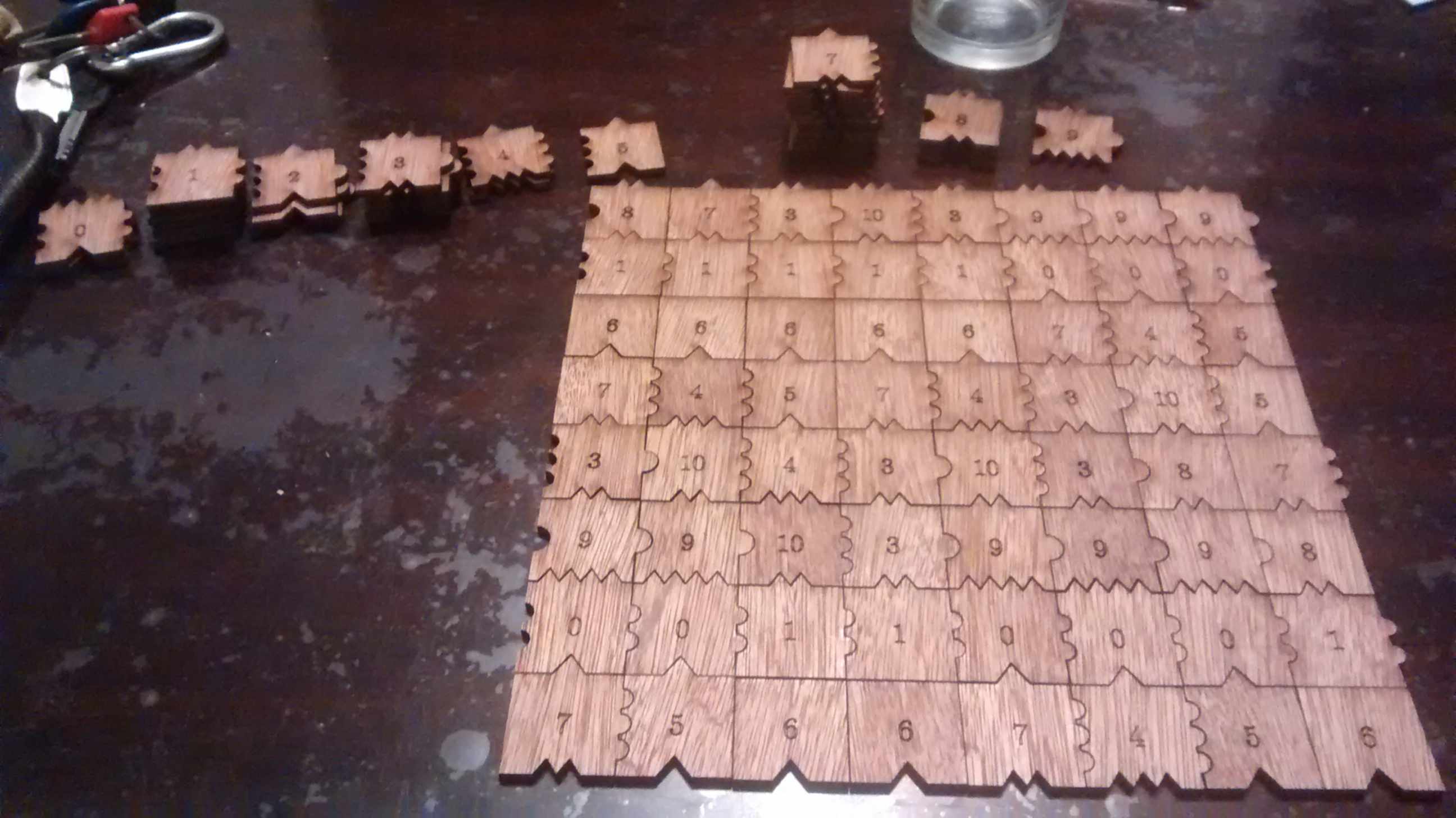
One may recreate the 33 x 19 tiling as follows (note that I am using Cartesian-like coordinates, so the first list data[0] actually is the first column from bottom to top):
sage: data = [[10, 4, 6, 1, 3, 3, 7, 0, 9, 7, 2, 6, 1, 3, 8, 7, 0, 9, 7],
....:  [4, 5, 6, 1, 8, 10, 4, 0, 9, 3, 8, 7, 0, 9, 7, 5, 0, 9, 3],
....:  [3, 7, 6, 1, 7, 2, 5, 0, 9, 8, 7, 5, 0, 9, 3, 7, 0, 9, 10],
....:  [10, 4, 6, 1, 3, 8, 7, 0, 9, 7, 5, 6, 1, 8, 10, 4, 0, 9, 3],
....:  [2, 5, 6, 1, 8, 7, 5, 0, 9, 3, 7, 6, 1, 7, 2, 5, 0, 9, 8],
....:  [8, 7, 6, 1, 7, 5, 6, 1, 8, 10, 4, 6, 1, 3, 8, 7, 0, 9, 7],
....:  [7, 5, 6, 1, 3, 7, 6, 1, 7, 2, 5, 6, 1, 8, 7, 5, 0, 9, 3],
....:  [3, 7, 6, 1, 10, 4, 6, 1, 3, 8, 7, 6, 1, 7, 5, 6, 1, 8, 10],
....:  [10, 4, 6, 1, 3, 3, 7, 0, 9, 7, 5, 6, 1, 3, 7, 6, 1, 7, 2],
....:  [2, 5, 6, 1, 8, 10, 4, 0, 9, 3, 7, 6, 1, 10, 4, 6, 1, 3, 8],
....:  [8, 7, 6, 1, 7, 5, 5, 0, 9, 10, 4, 6, 1, 3, 3, 7, 0, 9, 7],
....:  [7, 5, 6, 1, 3, 7, 6, 1, 10, 4, 5, 6, 1, 8, 10, 4, 0, 9, 3],
....:  [3, 7, 6, 1, 10, 4, 6, 1, 3, 3, 7, 6, 1, 7, 2, 5, 0, 9, 8],
....:  [10, 4, 6, 1, 3, 3, 7, 0, 9, 10, 4, 6, 1, 3, 8, 7, 0, 9, 7],
....:  [4, 5, 6, 1, 8, 10, 4, 0, 9, 3, 3, 7, 0, 9, 7, 5, 0, 9, 3],
....:  [3, 7, 6, 1, 7, 2, 5, 0, 9, 8, 10, 4, 0, 9, 3, 7, 0, 9, 10],
....:  [10, 4, 6, 1, 3, 8, 7, 0, 9, 7, 5, 5, 0, 9, 10, 4, 0, 9, 3],
....:  [2, 5, 6, 1, 8, 7, 5, 0, 9, 3, 7, 6, 1, 10, 4, 5, 0, 9, 8],
....:  [8, 7, 6, 1, 7, 5, 6, 1, 8, 10, 4, 6, 1, 3, 3, 7, 0, 9, 7],
....:  [7, 5, 6, 1, 3, 7, 6, 1, 7, 2, 5, 6, 1, 8, 10, 4, 0, 9, 3],
....:  [3, 7, 6, 1, 10, 4, 6, 1, 3, 8, 7, 6, 1, 7, 2, 5, 0, 9, 8],
....:  [10, 4, 6, 1, 3, 3, 7, 0, 9, 7, 2, 6, 1, 3, 8, 7, 0, 9, 7],
....:  [4, 5, 6, 1, 8, 10, 4, 0, 9, 3, 8, 7, 0, 9, 7, 5, 0, 9, 3],
....:  [3, 7, 6, 1, 7, 2, 5, 0, 9, 8, 7, 5, 0, 9, 3, 7, 0, 9, 10],
....:  [10, 4, 6, 1, 3, 8, 7, 0, 9, 7, 5, 6, 1, 8, 10, 4, 0, 9, 3],
....:  [3, 3, 7, 0, 9, 7, 5, 0, 9, 3, 7, 6, 1, 7, 2, 5, 0, 9, 8],
....:  [8, 10, 4, 0, 9, 3, 7, 0, 9, 10, 4, 6, 1, 3, 8, 7, 0, 9, 7],
....:  [7, 5, 5, 0, 9, 10, 4, 0, 9, 3, 3, 7, 0, 9, 7, 5, 0, 9, 3],
....:  [3, 7, 6, 1, 10, 4, 5, 0, 9, 8, 10, 4, 0, 9, 3, 7, 0, 9, 10],
....:  [10, 4, 6, 1, 3, 3, 7, 0, 9, 7, 5, 5, 0, 9, 10, 4, 0, 9, 3],
....:  [2, 5, 6, 1, 8, 10, 4, 0, 9, 3, 7, 6, 1, 10, 4, 5, 0, 9, 8],
....:  [8, 7, 6, 1, 7, 5, 5, 0, 9, 10, 4, 6, 1, 3, 3, 7, 0, 9, 7],
....:  [7, 5, 6, 1, 3, 7, 6, 1, 10, 4, 5, 6, 1, 8, 10, 4, 0, 9, 3]]
The above patch have been chosen among 1000 other randomly generated as the closest to the asymptotic frequencies of the tiles in Jeandel-Rao tilings (or at least in the minimal subshift that I describe in the preprint):
sage: from collections import Counter
sage: c = Counter(flatten(data))
sage: tile_count = [c[i] for i in range(11)]
The asymptotic frequencies:
sage: phi = golden_ratio.n()
sage: Linv = [2*phi + 6, 2*phi + 6, 18*phi + 10, 2*phi + 6, 8*phi + 2,
....:      5*phi + 4, 2*phi + 6, 12/5*phi + 14/5, 8*phi + 2,
....:      2*phi + 6, 8*phi + 2]
sage: perfect_proportions = vector([1/a for a in Linv])
Comparison of the number of tiles of each type with the expected frequency:
sage: header_row = ['tile id', 'Asymptotic frequency', 'Expected nb of copies',
....:               'Nb copies in the 33x19 patch']
sage: columns = [range(11), perfect_proportions, vector(perfect_proportions)*33*19, tile_count]
sage: table(columns=columns, header_row=header_row)
  tile id   Asymptotic frequency   Expected nb of copies   Nb copies in the 33x19 patch
+---------+----------------------+-----------------------+------------------------------+
  0         0.108271182329550      67.8860313206280        67
  1         0.108271182329550      67.8860313206280        65
  2         0.0255593590340479     16.0257181143480        16
  3         0.108271182329550      67.8860313206280        71
  4         0.0669152706817991     41.9558747174880        42
  5         0.0827118232955023     51.8603132062800        51
  6         0.108271182329550      67.8860313206280        65
  7         0.149627093977301      93.8161879237680        95
  8         0.0669152706817991     41.9558747174880        44
  9         0.108271182329550      67.8860313206280        67
  10        0.0669152706817991     41.9558747174880        44
I brought the \(33\times19=641\) tiles at the conference and offered to the first 7 persons to find a \(7\times 7\) tiling the opportunity to keep the 49 tiles they used. 49 is a good number since the frequency of the lowest tile (with id 2) is about 2% which allows to have at least one copy of each tile in a subset of 49 tiles allowing a solution.
A natural question to ask is how many such \(7\times 7\) tilings does there exist? With ticket #25125 that was merged in Sage 8.3 this Spring, it is possible to enumerate and count solutions in parallel with Knuth dancing links algorithm. After the installation of the Sage Optional package slabbe (sage -pip install slabbe), one may compute that there are 152244 solutions.
sage: from slabbe import WangTileSet
sage: tiles = [(2,4,2,1), (2,2,2,0), (1,1,3,1), (1,2,3,2), (3,1,3,3),
....: (0,1,3,1), (0,0,0,1), (3,1,0,2), (0,2,1,2), (1,2,1,4), (3,3,1,2)]
sage: T0 = WangTileSet(tiles)
sage: T0_solver = T0.solver(7,7)
sage: %time T0_solver.number_of_solutions(ncpus=8)
CPU times: user 16 ms, sys: 82.3 ms, total: 98.3 ms
Wall time: 388 ms
152244
One may also get the list of all solutions and print one of them:
sage: %time L = T0_solver.all_solutions(); print(len(L))
152244
CPU times: user 6.46 s, sys: 344 ms, total: 6.8 s
Wall time: 6.82 s
sage: L[0]
A wang tiling of a 7 x 7 rectangle
sage: L[0].table()  # warning: the output is in Cartesian-like coordinates
[[1, 8, 10, 4, 5, 0, 9],
 [1, 7, 2, 5, 6, 1, 8],
 [1, 3, 8, 7, 6, 1, 7],
 [0, 9, 7, 5, 6, 1, 3],
 [0, 9, 3, 7, 6, 1, 8],
 [1, 8, 10, 4, 6, 1, 7],
 [1, 7, 2, 2, 6, 1, 3]]
This is the number of distinct sets of 49 tiles which admits a 7x7 solution:
sage: from collections import Counter
sage: def count_tiles(tiling):
....:     C = Counter(flatten(tiling.table()))
....:     return tuple(C.get(a,0) for a in range(11))
sage: Lfreq = map(count_tiles, L)
sage: Lfreq_count = Counter(Lfreq)
sage: len(Lfreq_count)
83258
Number of other solutions with the same set of 49 tiles:
sage: Counter(Lfreq_count.values())
Counter({1: 49076, 2: 19849, 3: 6313, 4: 3664, 6: 1410, 5: 1341, 7: 705, 8:
293, 9: 159, 14: 116, 10: 104, 12: 97, 18: 44, 11: 26, 15: 24, 13: 10, 17: 8,
22: 6, 32: 6, 16: 3, 28: 2, 19: 1, 21: 1})
How the number of \(k\times k\)-solutions grows for k from 0 to 9:
sage: [T0.solver(k,k).number_of_solutions() for k in range(10)]
[0, 11, 85, 444, 1723, 9172, 50638, 152244, 262019, 1641695]
Unfortunately, most of those \(k\times k\)-solutions are not extendable to a tiling of the whole plane. Indeed the number of \(k\times k\) patches in the language of the minimal aperiodic subshift that I am able to describe and which is a proper subset of Jeandel-Rao tilings seems, according to some heuristic, to be something like:
[1, 11, 49, 108, 184, 268, 367, 483]
I do not share my (ugly) code for this computation yet, as I will rather share clean code soon when times come. So among the 152244 about only 483 (0.32%) of them are prolongable into a uniformly recurrent tiling of the plane.
slabbe-0.2.spkg released
30 novembre 2015 | Catégories: sage, slabbe spkg | View CommentsThese is a summary of the functionalities present in slabbe-0.2.spkg optional Sage package. It works on version 6.8 of Sage but will work best with sage-6.10 (it is using the new code for cartesian_product merged the the betas of sage-6.10). It contains 7 new modules:
- finite_word.py
- language.py
- lyapunov.py
- matrix_cocycle.py
- mult_cont_frac.pyx
- ranking_scale.py
- tikz_picture.py
Cheat Sheets
The best way to have a quick look at what can be computed with the optional Sage package slabbe-0.2.spkg is to look at the 3-dimensional Continued Fraction Algorithms Cheat Sheets available on the arXiv since today. It gathers a handful of informations on different 3-dimensional Continued Fraction Algorithms including well-known and old ones (Poincaré, Brun, Selmer, Fully Subtractive) and new ones (Arnoux-Rauzy-Poincaré, Reverse, Cassaigne).
Installation
sage -i http://www.slabbe.org/Sage/slabbe-0.2.spkg    # on sage 6.8
sage -p http://www.slabbe.org/Sage/slabbe-0.2.spkg    # on sage 6.9 or beyond
Examples
Computing the orbit of Brun algorithm on some input in \(\mathbb{R}^3_+\) including dual coordinates:
sage: from slabbe.mult_cont_frac import Brun
sage: algo = Brun()
sage: algo.cone_orbit_list((100, 87, 15), 4)
[(13.0, 87.0, 15.0, 1.0, 2.0, 1.0, 321),
 (13.0, 72.0, 15.0, 1.0, 2.0, 3.0, 132),
 (13.0, 57.0, 15.0, 1.0, 2.0, 5.0, 132),
 (13.0, 42.0, 15.0, 1.0, 2.0, 7.0, 132)]
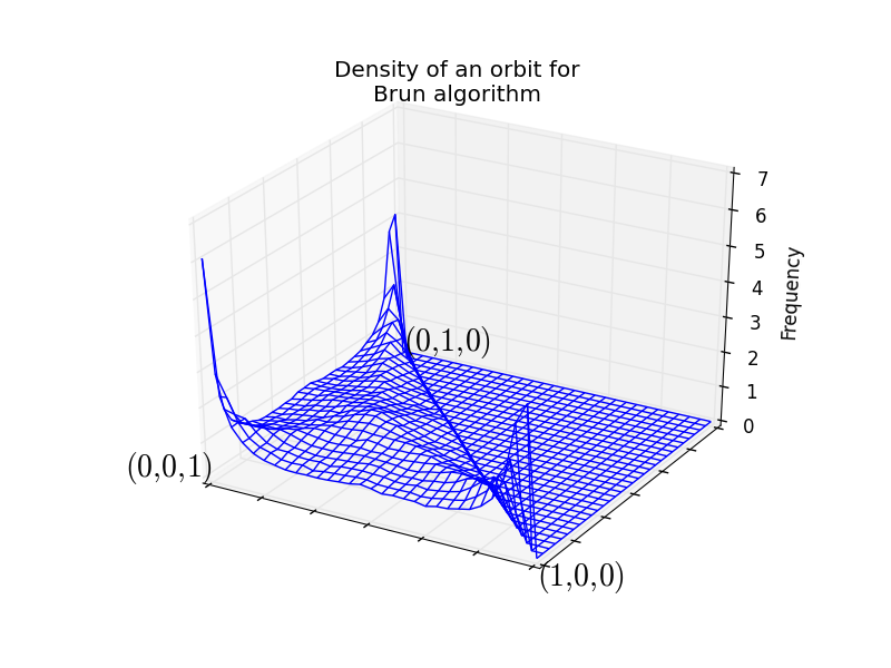
Computing the invariant measure:
sage: fig = algo.invariant_measure_wireframe_plot(n_iterations=10^6, ndivs=30)
sage: fig.savefig('a.png')
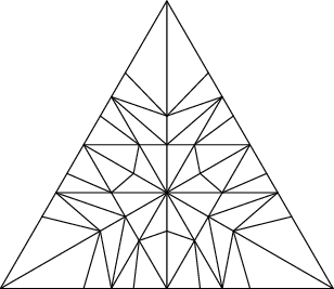
Drawing the cylinders:
sage: cocycle = algo.matrix_cocycle()
sage: t = cocycle.tikz_n_cylinders(3, scale=3)
sage: t.png()
Computing the Lyapunov exponents of the 3-dimensional Brun algorithm:
sage: from slabbe.lyapunov import lyapunov_table
sage: lyapunov_table(algo, n_orbits=30, n_iterations=10^7)
  30 succesful orbits     min       mean      max       std
+-----------------------+---------+---------+---------+---------+
  $\theta_1$              0.3026    0.3045    0.3051    0.00046
  $\theta_2$              -0.1125   -0.1122   -0.1115   0.00020
  $1-\theta_2/\theta_1$   1.3680    1.3684    1.3689    0.00024
Dealing with tikzpictures
Since I create lots of tikzpictures in my code and also because I was unhappy at how the view command of Sage handles them (a tikzpicture is not a math expression to put inside dollar signs), I decided to create a class for tikzpictures. I think this module could be useful in Sage so I will propose its inclusion soon.
I am using the standalone document class which allows some configurations like the border:
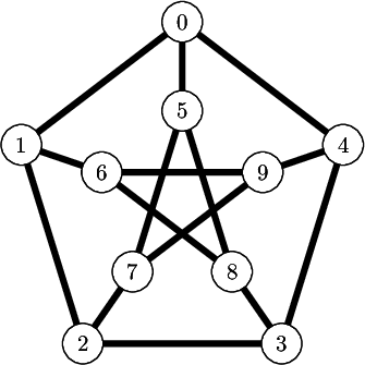
sage: from slabbe import TikzPicture
sage: g = graphs.PetersenGraph()
sage: s = latex(g)
sage: t = TikzPicture(s, standalone_configs=["border=4mm"], packages=['tkz-graph'])
The repr method does not print all of the string since it is often very long. Though it shows how many lines are not printed:
sage: t
\documentclass[tikz]{standalone}
\standaloneconfig{border=4mm}
\usepackage{tkz-graph}
\begin{document}
\begin{tikzpicture}
%
\useasboundingbox (0,0) rectangle (5.0cm,5.0cm);
%
\definecolor{cv0}{rgb}{0.0,0.0,0.0}
...
... 68 lines not printed (3748 characters in total) ...
...
\Edge[lw=0.1cm,style={color=cv6v8,},](v6)(v8)
\Edge[lw=0.1cm,style={color=cv6v9,},](v6)(v9)
\Edge[lw=0.1cm,style={color=cv7v9,},](v7)(v9)
%
\end{tikzpicture}
\end{document}
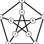
There is a method to generates a pdf and another for generating a png. Both opens the file in a viewer by default unless view=False:
sage: pathtofile = t.png(density=60, view=False)
sage: pathtofile = t.pdf()
Compare this with the output of view(s, tightpage=True) which does not allow to control the border and also creates a second empty page on some operating system (osx, only one page on ubuntu):
sage: view(s, tightpage=True)
One can also provide the filename where to save the file in which case the file is not open in a viewer:
sage: _ = t.pdf('petersen_graph.pdf')
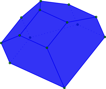
Another example with polyhedron code taken from this Sage thematic tutorial Draw polytopes in LateX using TikZ:
sage: V = [[1,0,1],[1,0,0],[1,1,0],[0,0,-1],[0,1,0],[-1,0,0],[0,1,1],[0,0,1],[0,-1,0]]
sage: P = Polyhedron(vertices=V).polar()
sage: s = P.projection().tikz([674,108,-731],112)
sage: t = TikzPicture(s)
sage: t
\documentclass[tikz]{standalone}
\begin{document}
\begin{tikzpicture}%
        [x={(0.249656cm, -0.577639cm)},
        y={(0.777700cm, -0.358578cm)},
        z={(-0.576936cm, -0.733318cm)},
        scale=2.000000,
...
... 80 lines not printed (4889 characters in total) ...
...
\node[vertex] at (1.00000, 1.00000, -1.00000)     {};
\node[vertex] at (1.00000, 1.00000, 1.00000)     {};
%%
%%
\end{tikzpicture}
\end{document}
sage: _ = t.pdf()
Next Page »
Propulsé par Blogofile
S'abonner au Flux RSS
et aux Commentaires.

This work by Sébastien Labbé is licensed under a Creative Commons Attribution-ShareAlike 4.0 International License.