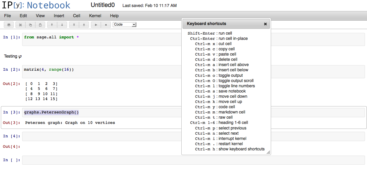
Demo of the IPython notebook at Sage Paris group meeting
06 mars 2014 | Catégories: ipython, sage | View CommentsToday I am presenting the IPython notebook at the meeting of the Sage Paris group. This post gathers what I prepared.
Installation
First you can install the ipython notebook in Sage as explained in this previous blog post. If everything works, then you run:
sage -ipython notebook
and this will open a browser.
Turn on Sage preparsing
Create a new notebook and type:
In [1]: 3 + 3
6
In [2]: 2 / 3
0
In [3]: matrix
Traceback (most recent call last):
...
NameError: name 'matrix' is not defined
By default, Sage preparsing is turn off and Sage commands are not known. To turn on the Sage preparsing (thanks to a post of Jason on sage-devel):
%load_ext sage.misc.sage_extension
Since sage-6.2, according to sage-devel, the command is:
%load_ext sage
You now get Sage commands working in ipython:
In [4]: 3 + 4
Out[4]: 7
In [5]: 2 / 3
Out[5]: 2/3
In [6]: type(_)
Out[6]: <type 'sage.rings.rational.Rational'>
In [7]: matrix(3, range(9))
Out[7]:
[0 1 2]
[3 4 5]
[6 7 8]
Scroll and hide output
If the output is too big, click on Out to scroll or hide the output:
In [8]: range(1000)
Sage 3d Graphics
3D graphics works but open in a new Jmol window:
In [9]: sphere()
Sage 2d Graphics
Similarly, 2D graphics works but open in a new window:
In [10]: plot(sin(x), (x,0,10))
Inline Matplotlib graphics
To create inline matplotlib graphics, the notebook must be started with this command:
sage -ipython notebook --pylab=inline
Then, a matplotlib plot can be drawn inline (example taken from this notebook):
import matplotlib.pyplot as plt
import numpy as np
x = np.linspace(0, 3*np.pi, 500)
plt.plot(x, np.sin(x**2))
plt.title('A simple chirp');
Or with:
%load http://matplotlib.org/mpl_examples/showcase/integral_demo.py
According to the previous cited notebook, it seems, that the inline mode can also be decided from the notebook using a magic command, but with my version of ipython (0.13.2), I get an error:
In [11]: %matplotlib inline
ERROR: Line magic function `%matplotlib` not found.
Use latex in a markdown cell
Change an input cell into a markdown cell and then you may use latex:
Test $\alpha+\beta+\gamma$
Output in latex
The output can be shown with latex and mathjax using the ipython display function:
from IPython.display import display, Math
def my_show(obj): return display(Math(latex(obj)))
y = 1 / (x^2+1)
my_show(y)
ipynb format
Create a new notebook with only one cell. Name it range_10 and save:
In [1]: range(10)
Out[1]: [0, 1, 2, 3, 4, 5, 6, 7, 8, 9]
The file range_10.ipynb is saved in the directory. You can also download it from File > Download as > IPython (.ipynb). Here is the content of the file range_10.ipynb:
{
 "metadata": {
  "name": "range_10"
 },
 "nbformat": 3,
 "nbformat_minor": 0,
 "worksheets": [
  {
   "cells": [
    {
     "cell_type": "code",
     "collapsed": false,
     "input": [
      "range(10)"
     ],
     "language": "python",
     "metadata": {},
     "outputs": [
      {
       "output_type": "pyout",
       "prompt_number": 1,
       "text": [
        "[0, 1, 2, 3, 4, 5, 6, 7, 8, 9]"
       ]
      }
     ],
     "prompt_number": 1
    },
    {
     "cell_type": "code",
     "collapsed": false,
     "input": [],
     "language": "python",
     "metadata": {},
     "outputs": []
    }
   ],
   "metadata": {}
  }
 ]
}
ipynb is just json
A ipynb file is written in json format. Below, we use json to open the file `range_10.ipynb as a Python dictionnary.
sage: s = open('range_10.ipynb','r').read()
sage: import json
sage: D = json.loads(s)
sage: type(D)
dict
sage: D.keys()
[u'nbformat', u'nbformat_minor', u'worksheets', u'metadata']
sage: D
{u'metadata': {u'name': u'range_10'},
 u'nbformat': 3,
 u'nbformat_minor': 0,
 u'worksheets': [{u'cells': [{u'cell_type': u'code',
     u'collapsed': False,
     u'input': [u'range(10)'],
     u'language': u'python',
     u'metadata': {},
     u'outputs': [{u'output_type': u'pyout',
       u'prompt_number': 1,
       u'text': [u'[0, 1, 2, 3, 4, 5, 6, 7, 8, 9]']}],
     u'prompt_number': 1},
    {u'cell_type': u'code',
     u'collapsed': False,
     u'input': [],
     u'language': u'python',
     u'metadata': {},
     u'outputs': []}],
   u'metadata': {}}]}
Load vaucanson.ipynb
Download the file vaucanson.ipynb from the last meeting of Paris Sage Users. You can view the complete demo including pictures of automaton even if you are not able to install vaucanson on your machine.
IPython notebook from a Python file
In a Python file, separate your code with the following line to create cells:
# <codecell>
For example, create the following Python file. Then, import it in the notebook. It will get translated to ipynb format automatically.
# -*- coding: utf-8 -*-
# <nbformat>3.0</nbformat>

# <codecell>

%load_ext sage.misc.sage_extension

# <codecell>

matrix(4, range(16))

# <codecell>

factor(2^40-1)
More conversion
Since release 1.0 of IPython, many conversion from ipynb to other format are possible (html, latex, slides, markdown, rst, python). Unfortunately, the version of IPython in Sage is still 0.13.2 as of today but the version 1.2.1 will be in sage-6.2.
Dessins et calculs d'orbites avec Sage d'une fonction associée à l'algo LLL
04 février 2014 | Catégories: sage | View CommentsAujourd'hui avait lieu une rencontre de l'ANR DynA3S. Suite à une présentation de Brigitte Vallée, j'ai codé quelques lignes en Sage pour étudier une fonction qu'elle a introduite. Cette fonction est reliée à la compréhension de la densité des termes sous-diagonaux dans l'exécution de l'algorithme LLL.
D'abord voici mon fichier: brigitte.sage.
Pour utiliser ce fichier, il faut d'abord l'importer dans Sage en utilisant la commande suivante. En ligne de commande, ça fonctionne bien. Dans le Sage notebook, je ne sais plus trop si la commande load permet encore de le faire (?):
sage: %runfile brigitte.sage # not tested
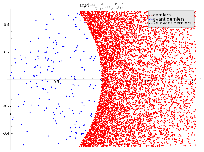
On doit générer plusieurs orbites pour visualiser quelque chose, car les orbites de la fonction sont de taille 1, 2 ou 3 en général avant que la condition d'arrêt soit atteinte. Ici, on génère 10000 orbites (les points initiaux sont choisis aléatoirement et uniformément dans \([0,1]\times[-0.5, 0.5]\). On dessine les derniers points des orbites:
sage: D = plusieurs_orbit(10000)
Note: la plus longue orbite est de taille 3
sage: A = points(D[0], color='red', legend_label='derniers')
sage: B = points(D[1], color='blue', legend_label='avant derniers')
sage: C = points(D[2], color='black', legend_label='2e avant derniers')
sage: G = A + B + C
sage: G.axes_labels(("$x$", r"$\nu$"))
sage: title = r"$(x,\nu) \mapsto (\frac{x}{(x+\nu^2)^2},\frac{\nu}{(x+\nu^2)})$"
sage: G.show(title=title, xmax=2)
Un raccourci pour faire à peu près le même dessin que ci-haut:
sage: draw_plusieurs_orbites(10000).show(xmax=2)
On dessine des histogrammes surperposés de la densité de ces points une fois projetés sur l'axe des \(\nu\):
sage: histogrammes_nu(10000, nbox=10)
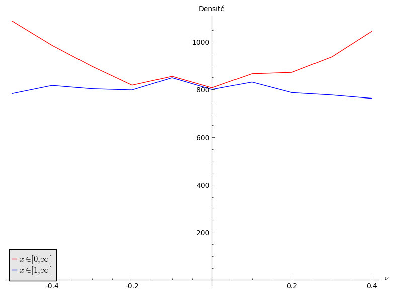
Le dessin semble indiquer que la densité non uniforme semble provenir simplement par les points \((x,\nu)\) tels que \(x\leq 1\).
On dessine des histogrammes superposés de la densité de ces points une fois projetés sur l'axe des \(x\) (on donne des couleurs selon la valeur de \(\nu\)):
sage: histogrammes_x(30000, nbox=5, ymax=1500, xmax=8)
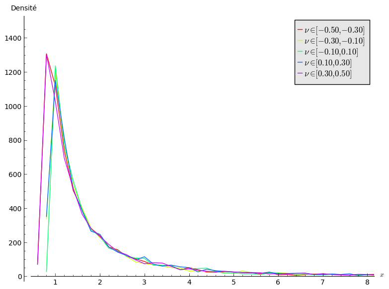
Le dessin semble indiquer que la densité ne dépend pas de \(\nu\) pour \(x\geq 1\).
Using sage in the new ipython notebook
10 février 2013 | Catégories: ipython, sage | View Comments(NEW: See also the demo I made at the Sage Paris group meeting in March 2014.)
Ticket #12719 (Upgrade to IPython 0.13) was merged into sage-5.7.beta1. This took a lot of energy (see the number of comments in the ticket and especially the number of patches and dependencies). Big thanks to Volker Braun, Mike Hansen, Jason Grout, Jeroen Demeyer who worked on this since almost one year. Note that in December 2012, the IPython project has received a $1.15M grant from the Alfred P. Sloan foundation, that will support IPython development for the next two years. I really like this IPython sage command line interface so it is really good news!
The IPython notebook
Since version 0.12 (December 21 2011), IPython is released with its own notebook. The differences with the Sage Notebook are explained by Fernando Perez, leader of IPython project, in the blog post The IPython notebook: a historical retrospective he wrote in January 2012. One of the differences is that the IPython Notebook run in its own directory whereas each cell of the Sage Notebook lives in its directory. As William Stein says in the presentation Browser-based notebook interfaces for mathematical software - past, present and future he gave last December at ICERM, there are plenty of projects and directions these days for those interfaces.
In May 2012, I tested the same ticket which was to upgrade to IPython 0.12 at that time. Today, I was curious to test it again.
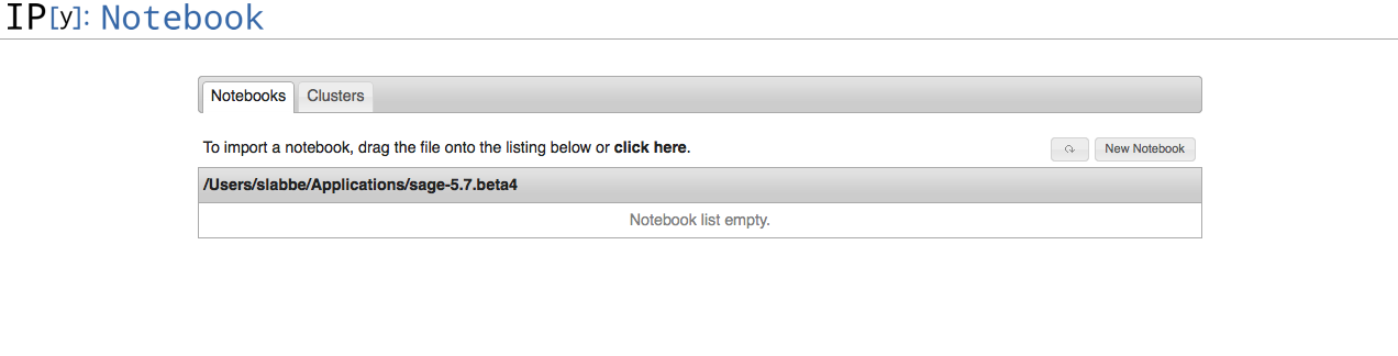
First, I installed sage-5.7.beta4:
./sage -version
Sage Version 5.7.beta4, Release Date: 2013-02-09
Install tornado:
./sage -sh
easy_install-2.7 tornado
[update March 6th, 2014] Note that some linux user have to install libssl-dev before tornado:
sudo apt-get install libssl-dev
Install zeromq and pyzmq:
./sage -i zeromq
./sage -i pyzmq
Start the ipython notebook:
./sage -ipython notebook
[NotebookApp] Using existing profile dir: u'/Users/slabbe/.sage/ipython-0.12/profile_default'
[NotebookApp] Serving notebooks from /Users/slabbe/Applications/sage-5.7.beta4
[NotebookApp] The IPython Notebook is running at: http://127.0.0.1:8888/
[NotebookApp] Use Control-C to stop this server and shut down all kernels.
Create a new notebook. One may use sage commands by adding the line from sage.all import * in the first cell.
The next things I want to look at are:
- Test the conversion of files from .py to .pynb.
- Test the conversion of files from .rst to .pynb.
- Test the qtconsole.
- Test the parallel computing capacities of the IPython.
Understanding Python class inheritance and Sage coding convention with fruits
28 janvier 2013 | Catégories: python, sage | View CommentsSince Sage Days 20 at Marseille held in January 2010, I have been doing the same example over and over again each time I showed someone else how object oriented coding works in Python: using fruits, strawberry, oranges and bananas.
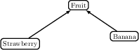
Here is my file: fruit.py. I use to build it from scratch by adding one line at a time using attach command to see what has changed starting with Banana class, then Strawberry class then Fruit class which gathers all common methods.
This time, I wrote the complete documentation (all tests pass, coverage is 100%) and followed Sage coding convention as far as I know them. Thus, I hope this file can be useful as an example to explain those coding convention to newcomers.
One may check that all tests pass using:
$ sage -t fruit.py
sage -t  "fruit.py"
[3.7 s]

----------------------------------------------------------------------
All tests passed!
Total time for all tests: 3.8 seconds
One may check that documentation and doctest coverage is 100%:
$ sage -coverage fruit.py
----------------------------------------------------------------------
fruit.py
SCORE fruit.py: 100% (10 of 10)
----------------------------------------------------------------------
Python function vs Symbolic function in Sage
21 janvier 2013 | Catégories: sage | View CommentsThis message is about differences between a Python function and a symbolic function. This is also explained in the Some Common Issues with Functions page in the Sage Tutorial.
In Sage, one may define a symbolic function like:
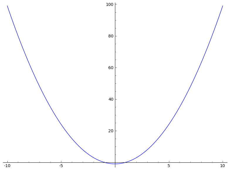
sage: f(x) = x^2-1
And draw it using one the following way (both works):
sage: plot(f, (x,-10,10))
sage: plot(f(x), (x,-10,10))
Here both f and f(x) are symbolic expressions:
sage: type(f)
<type 'sage.symbolic.expression.Expression'>
sage: type(f(x))
<type 'sage.symbolic.expression.Expression'>
although there are different:
sage: f
x |--> x^2 - 1
sage: f(x)
x^2 - 1
Now if f is a Python function defined with a def statement:
sage: def f(x):
....:     if x>0:
....:         return x
....:     else:
....:         return 0
It is really a Python function:
sage: f
<function f at 0xb933470>
sage: type(f)
<type 'function'>
As above, one can draw the function f:
sage: plot(f, (x,-10,10))
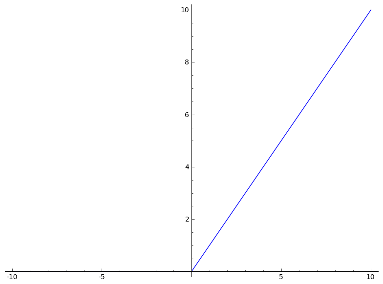
But be carefull, drawing f(x) will not work as expected:
sage: plot(f(x), (x,-10,10))
Why? Because, the python function f gets evaluated on the variable x and this may either raise an exception depending on the definition of f or return some result which might not be a symbolic expression. Here f(x) gets always evaluated to zero because in the definition of f, bool(x > 0) returns False:
sage: x
x
sage: bool(x > 0)
False
sage: f(x)
0
Hence the following constant function is drawn:
sage: plot(0, (x,-10,10))
which is not what we want.
« Previous Page -- Next Page »
Propulsé par Blogofile
S'abonner au Flux RSS
et aux Commentaires.

This work by Sébastien Labbé is licensed under a Creative Commons Attribution-ShareAlike 4.0 International License.