Arnoux-Rauzy-Poincaré sequences
26 février 2015 | Catégories: sage | View CommentsIn a recent article with Valérie Berthé [BL15], we provided a multidimensional continued fraction algorithm called Arnoux-Rauzy-Poincaré (ARP) to construct, given any vector \(v\in\mathbb{R}_+^3\), an infinite word \(w\in\{1,2,3\}^\mathbb{N}\) over a three-letter alphabet such that the frequencies of letters in \(w\) exists and are equal to \(v\) and such that the number of factors (i.e. finite block of consecutive letters) of length \(n\) appearing in \(w\) is linear and less than \(\frac{5}{2}n+1\). We also conjecture that for almost all \(v\) the contructed word describes a discrete path in the positive octant staying at a bounded distance from the euclidean line of direction \(v\).
In Sage, you can construct this word using the next version of my package slabbe-0.2 (not released yet, email me to press me to finish it). The one with frequencies of letters proportionnal to \((1, e, \pi)\) is:
sage: from slabbe.mcf import algo
sage: D = algo.arp.substitutions()
sage: it = algo.arp.coding_iterator((1,e,pi))
sage: w = words.s_adic(it, repeat(1), D)
word: 1232323123233231232332312323123232312323...
The factor complexity is close to 2n+1 and the balance is often less or equal to three:
sage: w[:10000].number_of_factors(100)
202
sage: w[:100000].number_of_factors(1000)
2002
sage: w[:1000].balance()
3
sage: w[:2000].balance()
3
Note that bounded distance from the euclidean line almost surely was proven in [DHS2013] for Brun algorithm, another MCF algorithm.
Other approaches: Standard model and billiard sequences
Other approaches have been proposed to construct such discrete lines.
One of them is the standard model of Eric Andres [A03]. It is also equivalent to billiard sequences in the cube. It is well known that the factor complexity of billiard sequences is quadratic \(p(n)=n^2+n+1\) [AMST94]. Experimentally, we can verify this. We first create a billiard word of some given direction:
sage: from slabbe import BilliardCube
sage: v = vector(RR, (1, e, pi))
sage: b = BilliardCube(v)
sage: b
Cubic billiard of direction (1.00000000000000, 2.71828182845905, 3.14159265358979)
sage: w = b.to_word()
sage: w
word: 3231232323123233213232321323231233232132...
We create some prefixes of \(w\) that we represent internally as char*. The creation is slow because the implementation of billiard words in my optional package is in Python and is not that efficient:
sage: p3 = Word(w[:10^3], alphabet=[1,2,3], datatype='char')
sage: p4 = Word(w[:10^4], alphabet=[1,2,3], datatype='char') # takes 3s
sage: p5 = Word(w[:10^5], alphabet=[1,2,3], datatype='char') # takes 32s
sage: p6 = Word(w[:10^6], alphabet=[1,2,3], datatype='char') # takes 5min 20s
We see below that exactly \(n^2+n+1\) factors of length \(n<20\) appears in the prefix of length 1000000 of \(w\):
sage: A = ['n'] + range(30)
sage: c3 = ['p_(w[:10^3])(n)'] + map(p3.number_of_factors, range(30))
sage: c4 = ['p_(w[:10^4])(n)'] + map(p4.number_of_factors, range(30))
sage: c5 = ['p_(w[:10^5])(n)'] + map(p5.number_of_factors, range(30)) # takes 4s
sage: c6 = ['p_(w[:10^6])(n)'] + map(p6.number_of_factors, range(30)) # takes 49s
sage: ref = ['n^2+n+1'] + [n^2+n+1 for n in range(30)]
sage: T = table(columns=[A,c3,c4,c5,c6,ref])
sage: T
  n    p_(w[:10^3])(n)   p_(w[:10^4])(n)   p_(w[:10^5])(n)   p_(w[:10^6])(n)   n^2+n+1
+----+-----------------+-----------------+-----------------+-----------------+---------+
  0    1                 1                 1                 1                 1
  1    3                 3                 3                 3                 3
  2    7                 7                 7                 7                 7
  3    13                13                13                13                13
  4    21                21                21                21                21
  5    31                31                31                31                31
  6    43                43                43                43                43
  7    52                55                56                57                57
  8    63                69                71                73                73
  9    74                85                88                91                91
  10   87                103               107               111               111
  11   100               123               128               133               133
  12   115               145               151               157               157
  13   130               169               176               183               183
  14   144               195               203               211               211
  15   160               223               232               241               241
  16   176               253               263               273               273
  17   192               285               296               307               307
  18   208               319               331               343               343
  19   224               355               368               381               381
  20   239               392               407               421               421
  21   254               430               448               463               463
  22   268               470               491               507               507
  23   282               510               536               553               553
  24   296               552               583               601               601
  25   310               596               632               651               651
  26   324               642               683               703               703
  27   335               687               734               757               757
  28   345               734               787               813               813
  29   355               783               842               871               871
Billiard sequences generate paths that are at a bounded distance from an euclidean line. This is equivalent to say that the balance is finite. The balance is defined as the supremum value of difference of the number of apparition of a letter in two factors of the same length. For billiard sequences, the balance is 2:
sage: p3.balance()
2
sage: p4.balance() # takes 2min 37s
2
Other approaches: Melançon and Reutenauer
Melançon and Reutenauer [MR13] also suggested a method that generalizes Christoffel words in higher dimension. The construction is based on the application of two substitutions generalizing the construction of sturmian sequences. Below we compute the factor complexity and the balance of some of their words over a three-letter alphabet.
On a three-letter alphabet, the two morphisms are:
sage: L = WordMorphism('1->1,2->13,3->2')
sage: R = WordMorphism('1->13,2->2,3->3')
sage: L
WordMorphism: 1->1, 2->13, 3->2
sage: R
WordMorphism: 1->13, 2->2, 3->3
Example 1: periodic case \(LRLRLRLRLR\dots\). In this example, the factor complexity seems to be around \(p(n)=2.76n\) and the balance is at least 28:
sage: from itertools import repeat, cycle
sage: W = words.s_adic(cycle((L,R)),repeat('1'))
sage: W
word: 1213122121313121312212212131221213131213...
sage: map(W[:10000].number_of_factors, [10,20,40,80])
[27, 54, 110, 221]
sage: [27/10., 54/20., 110/40., 221/80.]
[2.70000000000000, 2.70000000000000, 2.75000000000000, 2.76250000000000]
sage: W[:1000].balance()  # takes 1.6s
21
sage: W[:2000].balance()  # takes 6.4s
28
Example 2: \(RLR^2LR^4LR^8LR^{16}LR^{32}LR^{64}LR^{128}\dots\) taken from the conclusion of their article. In this example, the factor complexity seems to be \(p(n)=3n\) and balance at least as high (=bad) as \(122\):
sage: W = words.s_adic([R,L,R,R,L,R,R,R,R,L]+[R]*8+[L]+[R]*16+[L]+[R]*32+[L]+[R]*64+[L]+[R]*128,'1')
sage: W.length()
330312
sage: map(W.number_of_factors, [10, 20, 100, 200, 300, 1000])
[29, 57, 295, 595, 895, 2981]
sage: [29/10., 57/20., 295/100., 595/200., 895/300., 2981/1000.]
[2.90000000000000,
 2.85000000000000,
 2.95000000000000,
 2.97500000000000,
 2.98333333333333,
 2.98100000000000]
sage: W[:1000].balance()  # takes 1.6s
122
sage: W[:2000].balance()  # takes 6s
122
Example 3: some random ones. The complexity \(p(n)/n\) occillates between 2 and 3 for factors of length \(n=1000\) in prefixes of length 100000:
sage: for _ in range(10):
....:     W = words.s_adic([choice((L,R)) for _ in range(50)],'1')
....:     print W[:100000].number_of_factors(1000)/1000.
2.02700000000000
2.23600000000000
2.74000000000000
2.21500000000000
2.78700000000000
2.52700000000000
2.85700000000000
2.33300000000000
2.65500000000000
2.51800000000000
For ten randomly generated words, the balance goes from 6 to 27 which is much more than what is obtained for billiard words or by our approach:
sage: for _ in range(10):
....:     W = words.s_adic([choice((L,R)) for _ in range(50)],'1')
....:     print W[:1000].balance(), W[:2000].balance()
12 15
8 24
14 14
5 11
17 17
14 14
6 6
19 27
9 16
12 12
References
| [BL15] | V. Berthé, S. Labbé, Factor Complexity of S-adic words generated by the Arnoux-Rauzy-Poincaré Algorithm, Advances in Applied Mathematics 63 (2015) 90-130. http://dx.doi.org/10.1016/j.aam.2014.11.001 |
| [DHS2013] | Delecroix, Vincent, Tomás Hejda, and Wolfgang Steiner. “Balancedness of Arnoux-Rauzy and Brun Words.” In Combinatorics on Words, 119–31. Springer, 2013. http://link.springer.com/chapter/10.1007/978-3-642-40579-2_14. |
| [A03] | E. Andres, Discrete linear objects in dimension n: the standard model, Graphical Models 65 (2003) 92-111. |
| [AMST94] | P. Arnoux, C. Mauduit, I. Shiokawa, J. I. Tamura, Complexity of sequences defined by billiards in the cube, Bull. Soc. Math. France 122 (1994) 1-12. |
| [MR13] | G. Melançon, C. Reutenauer, On a class of Lyndon words extending Christoffel words and related to a multidimensional continued fraction algorithm. J. Integer Seq. 16, No. 9, Article 13.9.7, 30 p., electronic only (2013). https://cs.uwaterloo.ca/journals/JIS/VOL16/Reutenauer/reut3.html |
Abelian complexity of the Oldenburger sequence
27 septembre 2014 | Catégories: sage | View CommentsThe Oldenburger infinite sequence [O39] \[ K = 1221121221221121122121121221121121221221\ldots \] also known under the name of Kolakoski, is equal to its exponent trajectory. The exponent trajectory \(\Delta\) can be obtained by counting the lengths of blocks of consecutive and equal letters: \[ K = 1^12^21^22^11^12^21^12^21^22^11^22^21^12^11^22^11^12^21^22^11^22^11^12^21^12^21^22^11^12^21^12^11^22^11^22^21^12^21^2\ldots \] The sequence of exponents above gives the exponent trajectory of the Oldenburger sequence: \[ \Delta = 12211212212211211221211212\ldots \] which is equal to the original sequence \(K\). You can define this sequence in Sage:
sage: K = words.KolakoskiWord()
sage: K
word: 1221121221221121122121121221121121221221...
sage: K.delta()          # delta returns the exponent trajectory
word: 1221121221221121122121121221121121221221...
There are a lot of open problem related to basic properties of that sequence. For example, we do not know if that sequence is recurrent, that is, all finite subword or factor (finite block of consecutive letters) always reappear. Also, it is still open to prove whether the density of 1 in that sequence is equal to \(1/2\).
In this blog post, I do some computations on its abelian complexity \(p_{ab}(n)\) defined as the number of distinct abelian vectors of subwords of length \(n\) in the sequence. The abelian vector \(\vec{w}\) of a word \(w\) counts the number of occurences of each letter: \[ w = 12211212212 \quad \mapsto \quad 1^5 2^7 \text{, abelianized} \quad \mapsto \quad \vec{w} = (5, 7) \text{, the abelian vector of } w \]
Here are the abelian vectors of subwords of length 10 and 20 in the prefix of length 100 of the Oldenburger sequence. The functions abelian_vectors and abelian_complexity are not in Sage as of now. Code is available at trac #17058 to be merged in Sage soon:
sage: prefix = words.KolakoskiWord()[:100]
sage: prefix.abelian_vectors(10)
{(4, 6), (5, 5), (6, 4)}
sage: prefix.abelian_vectors(20)
{(8, 12), (9, 11), (10, 10), (11, 9), (12, 8)}
Therefore, the prefix of length 100 has 3 vectors of subwords of length 10 and 5 vectors of subwords of length 20:
sage: p100.abelian_complexity(10)
3
sage: p100.abelian_complexity(20)
5
I import the OldenburgerSequence from my optional spkg because it is faster than the implementation in Sage:
sage: from slabbe import KolakoskiWord as OldenburgerSequence
sage: Olden = OldenburgerSequence()
I count the number of abelian vectors of subwords of length 100 in the prefix of length \(2^{20}\) of the Oldenburger sequence:
sage: prefix = Olden[:2^20]
sage: %time prefix.abelian_vectors(100)
CPU times: user 3.48 s, sys: 66.9 ms, total: 3.54 s
Wall time: 3.56 s
{(47, 53), (48, 52), (49, 51), (50, 50), (51, 49), (52, 48), (53, 47)}
Number of abelian vectors of subwords of length less than 100 in the prefix of length \(2^{20}\) of the Oldenburger sequence:
sage: %time L100 = map(prefix.abelian_complexity, range(100))
CPU times: user 3min 20s, sys: 1.08 s, total: 3min 21s
Wall time: 3min 23s
sage: from collections import Counter
sage: Counter(L100)
Counter({5: 26, 6: 26, 4: 17, 7: 15, 3: 8, 8: 4, 2: 3, 1: 1})
Let's draw that:
sage: labels = ('Length of factors', 'Number of abelian vectors')
sage: title = 'Abelian Complexity of the prefix of length $2^{20}$ of Oldenburger sequence'
sage: list_plot(L100, color='green', plotjoined=True, axes_labels=labels, title=title)
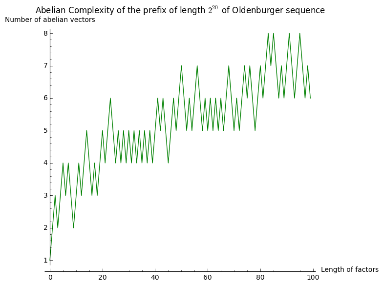
It seems to grow something like \(\log(n)\). Let's now consider subwords of length \(2^n\) for \(0\leq n\leq 12\) in the same prefix of length \(2^{20}\):
sage: %time L20 = [(2^n, prefix.abelian_complexity(2^n)) for n in range(20)]
CPU times: user 41 s, sys: 239 ms, total: 41.2 s
Wall time: 41.5 s
sage: L20
[(1, 2), (2, 3), (4, 3), (8, 3), (16, 3), (32, 5), (64, 5), (128, 9),
(256, 9), (512, 13), (1024, 17), (2048, 22), (4096, 27), (8192, 40),
(16384, 46), (32768, 67), (65536, 81), (131072, 85), (262144, 90), (524288, 104)]
I now look at subwords of length \(2^n\) for \(0\leq n\leq 23\) in the longer prefix of length \(2^{24}\):
sage: prefix = Olden[:2^24]
sage: %time L24 = [(2^n, prefix.abelian_complexity(2^n)) for n in range(24)]
CPU times: user 20min 47s, sys: 13.5 s, total: 21min
Wall time: 20min 13s
sage: L24
[(1, 2), (2, 3), (4, 3), (8, 3), (16, 3), (32, 5), (64, 5), (128, 9), (256,
9), (512, 13), (1024, 17), (2048, 23), (4096, 33), (8192, 46), (16384, 58),
(32768, 74), (65536, 98), (131072, 134), (262144, 165), (524288, 229),
(1048576, 302), (2097152, 371), (4194304, 304), (8388608, 329)]
The next graph gather all of the above computations:
sage: G = Graphics()
sage: legend = 'in the prefix of length 2^{}'
sage: G += list_plot(L24, plotjoined=True, thickness=4, color='blue', legend_label=legend.format(24))
sage: G += list_plot(L20, plotjoined=True, thickness=4, color='red', legend_label=legend.format(20))
sage: G += list_plot(L100, plotjoined=True, thickness=4, color='green', legend_label=legend.format(20))
sage: labels = ('Length of factors', 'Number of abelian vectors')
sage: title = 'Abelian complexity of Oldenburger sequence'
sage: G.show(scale=('semilogx', 2), axes_labels=labels, title=title)
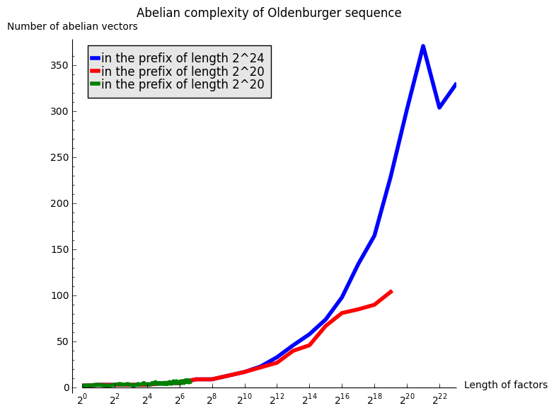
A linear growth in the above graphics with logarithmic \(x\) abcisse would mean a growth in \(\log(n)\). After those experimentations, my hypothesis is that the abelian complexity of the Oldenburger sequence grows like \(\log(n)^2\).
References
| [O39] | Oldenburger, Rufus (1939). "Exponent trajectories in symbolic dynamics". Transactions of the American Mathematical Society 46: 453–466. doi:10.2307/1989933 |
slabbe-0.1.spkg released
27 août 2014 | Catégories: sage, slabbe spkg | View CommentsThese is a summary of the functionalities present in slabbe-0.1 optional Sage package. It depends on version 6.3 of Sage because it uses RecursivelyEnumeratedSet code that was merged in 6.3. It contains modules on digital geometry, combinatorics on words and more.
Install the optional spkg (depends on sage-6.3):
sage -i http://www.liafa.univ-paris-diderot.fr/~labbe/Sage/slabbe-0.1.spkg
In each of the example below, you first have to import the module once and for all:
sage: from slabbe import *
To construct the image below, make sure to use tikz package so that view is able to compile tikz code when called:
sage: latex.add_to_preamble("\\usepackage{tikz}")
sage: latex.extra_preamble()
'\\usepackage{tikz}'
Draw the part of a discrete plane
sage: p = DiscretePlane([1,pi,7], 1+pi+7, mu=0)
sage: d = DiscreteTube([-5,5],[-5,5])
sage: I = p & d
sage: I
Intersection of the following objects:
Set of points x in ZZ^3 satisfying: 0 <= (1, pi, 7) . x + 0 < pi + 8
DiscreteTube: Preimage of [-5, 5] x [-5, 5] by a 2 by 3 matrix
sage: clip = d.clip()
sage: tikz = I.tikz(clip=clip)
sage: view(tikz, tightpage=True)

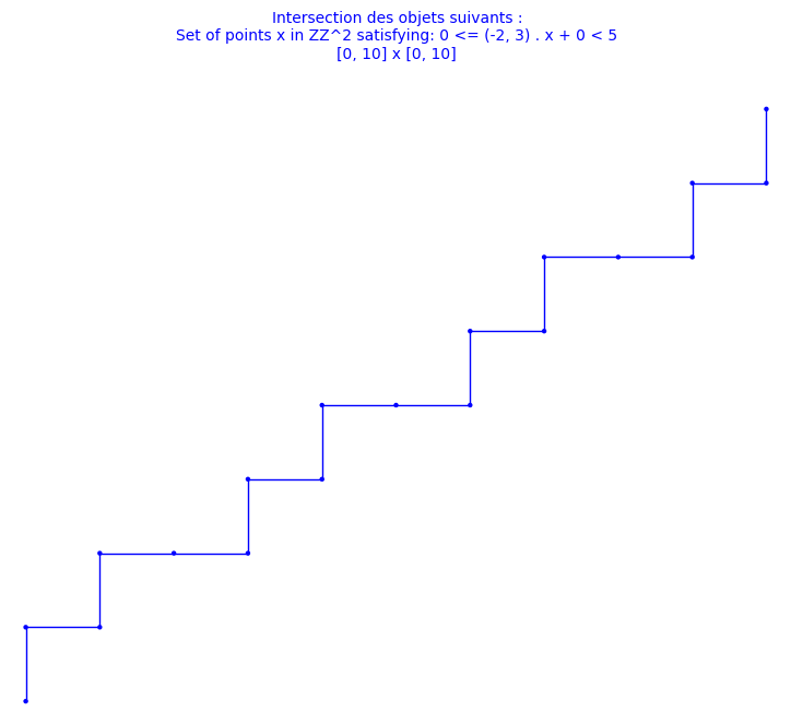
Draw the part of a discrete line
sage: L = DiscreteLine([-2,3], 5)
sage: b = DiscreteBox([0,10], [0,10])
sage: I = L & b
sage: I
Intersection of the following objects:
Set of points x in ZZ^2 satisfying: 0 <= (-2, 3) . x + 0 < 5
[0, 10] x [0, 10]
sage: I.plot()
Double square tiles
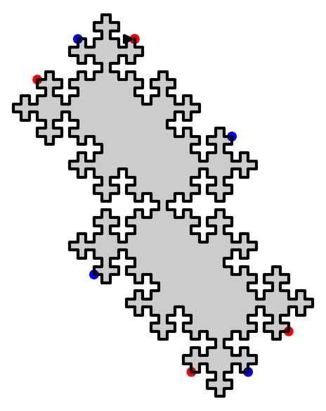
This module was developped for the article on the combinatorial properties of double square tiles written with Ariane Garon and Alexandre Blondin Massé [BGL2012]. The original version of the code was written with Alexandre.
sage: D = DoubleSquare((34,21,34,21))
sage: D
Double Square Tile
  w0 = 3032321232303010303230301012101030   w4 = 1210103010121232121012123230323212
  w1 = 323030103032321232303                w5 = 101212321210103010121
  w2 = 2321210121232303232123230301030323   w6 = 0103032303010121010301012123212101
  w3 = 212323032321210121232                w7 = 030101210103032303010
(|w0|, |w1|, |w2|, |w3|) = (34, 21, 34, 21)
(d0, d1, d2, d3)         = (42, 68, 42, 68)
(n0, n1, n2, n3)         = (0, 0, 0, 0)
sage: D.plot()
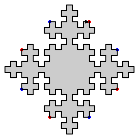
sage: D.extend(0).extend(1).plot()
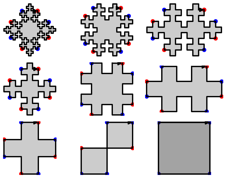
We have shown that using two invertible operations (called SWAP and TRIM), every double square tiles can be reduced to the unit square:
sage: D.plot_reduction()
The reduction operations are:
sage: D.reduction()
['SWAP_1', 'TRIM_1', 'TRIM_3', 'SWAP_1', 'TRIM_1', 'TRIM_3', 'TRIM_0', 'TRIM_2']
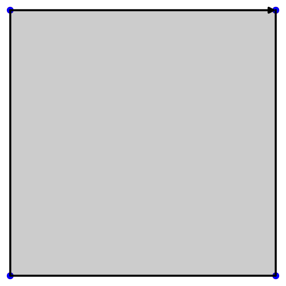
The result of the reduction is the unit square:
sage: unit_square = D.apply(D.reduction())
sage: unit_square
Double Square Tile
  w0 =     w4 =
  w1 = 3   w5 = 1
  w2 =     w6 =
  w3 = 2   w7 = 0
(|w0|, |w1|, |w2|, |w3|) = (0, 1, 0, 1)
(d0, d1, d2, d3)         = (2, 0, 2, 0)
(n0, n1, n2, n3)         = (0, NaN, 0, NaN)
sage: unit_square.plot()
Since SWAP and TRIM are invertible operations, we can recover every double square from the unit square:
sage: E = unit_square.extend(2).extend(0).extend(3).extend(1).swap(1).extend(3).extend(1).swap(1)
sage: D == E
True
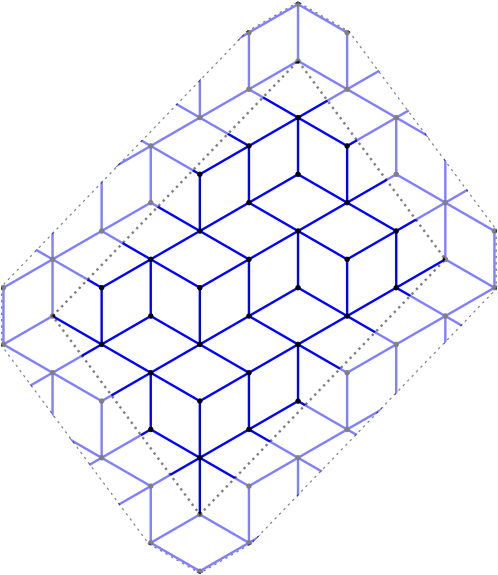
Christoffel graphs
This module was developped for the article on a d-dimensional extension of Christoffel Words written with Christophe Reutenauer [LR2014].
sage: G = ChristoffelGraph((6,10,15))
sage: G
Christoffel set of edges for normal vector v=(6, 10, 15)
sage: tikz = G.tikz_kernel()
sage: view(tikz, tightpage=True)
Bispecial extension types
This module was developped for the article on the factor complexity of infinite sequences genereated by substitutions written with Valérie Berthé [BL2014].
The extension type of an ordinary bispecial factor:
sage: L = [(1,3), (2,3), (3,1), (3,2), (3,3)]
sage: E = ExtensionType1to1(L, alphabet=(1,2,3))
sage: E
  E(w)   1   2   3
   1             X
   2             X
   3     X   X   X
 m(w)=0, ordinary
sage: E.is_ordinaire()
True
Creation of a strong-weak pair of bispecial words from a neutral not ordinaire word:
sage: p23 = WordMorphism({1:[1,2,3],2:[2,3],3:[3]})
sage: e = ExtensionType1to1([(1,2),(2,3),(3,1),(3,2),(3,3)], [1,2,3])
sage: e
  E(w)   1   2   3
   1         X
   2             X
   3     X   X   X
 m(w)=0, not ord.
sage: A,B = e.apply(p23)
sage: A
  E(3w)   1   2   3
    1
    2         X   X
    3     X   X   X
 m(w)=1, not ord.
sage: B
  E(23w)   1   2   3
    1          X
    2
    3              X
 m(w)=-1, not ord.
Fast Kolakoski word
This module was written for fun. It uses cython implementation inspired from the 10 lines of C code written by Dominique Bernardi and shared during Sage Days 28 in Orsay, France, in January 2011.
sage: K = KolakoskiWord()
sage: K
word: 1221121221221121122121121221121121221221...
sage: %time K[10^5]
CPU times: user 1.56 ms, sys: 7 µs, total: 1.57 ms
Wall time: 1.57 ms
1
sage: %time K[10^6]
CPU times: user 15.8 ms, sys: 30 µs, total: 15.8 ms
Wall time: 15.9 ms
2
sage: %time K[10^8]
CPU times: user 1.58 s, sys: 2.28 ms, total: 1.58 s
Wall time: 1.59 s
1
sage: %time K[10^9]
CPU times: user 15.8 s, sys: 12.4 ms, total: 15.9 s
Wall time: 15.9 s
1
This is much faster than the Python implementation available in Sage:
sage: K = words.KolakoskiWord()
sage: %time K[10^5]
CPU times: user 779 ms, sys: 25.9 ms, total: 805 ms
Wall time: 802 ms
1
References
| [BGL2012] | A. Blondin Massé, A. Garon, S. Labbé, Combinatorial properties of double square tiles, Theoretical Computer Science 502 (2013) 98-117. doi:10.1016/j.tcs.2012.10.040 |
| [LR2014] | Labbé, Sébastien, and Christophe Reutenauer. A d-dimensional Extension of Christoffel Words. arXiv:1404.4021 (April 15, 2014). |
| [BL2014] | V. Berthé, S. Labbé, Factor Complexity of S-adic sequences generated by the Arnoux-Rauzy-Poincaré Algorithm. arXiv:1404.4189 (April, 2014). |
Releasing slabbe, my own Sage package
27 août 2014 | Catégories: sage, slabbe spkg | View CommentsSince two years I wrote thousands of line of private code for my own research. Each module having between 500 and 2000 lines of code. The code which is the more clean corresponds to code written in conjunction with research articles. People who know me know that I systematically put docstrings and doctests in my code to facilitate reuse of the code by myself, but also in the idea of sharing it and eventually making it public.
I did not made that code into Sage because it was not mature enough. Also, when I tried to make a complete module go into Sage (see #13069 and #13346), then the monstrous never evolving #12224 became a dependency of the first and the second was unofficially reviewed asking me to split it into smaller chunks to make the review process easier. I never did it because I spent already too much time on it (making a module 100% doctested takes time). Also, the module was corresponding to a published article and I wanted to leave it just like that.
Getting new modules into Sage is hard
In general, the introduction of a complete new module into Sage is hard especially for beginners. Here are two examples I feel responsible for: #10519 is 4 years old and counting, the author has a new work and responsabilities; in #12996, the author was decouraged by the amount of work given by the reviewers. There is a lot of things a beginner has to consider to obtain a positive review. And even for a more advanced developper, other difficulties arise. Indeed, a module introduces a lot of new functions and it may also introduce a lot of new bugs... and Sage developpers are sometimes reluctant to give it a positive review. And if it finally gets a positive review, it is not available easily to normal users of Sage until the next release of Sage.
Releasing my own Sage package
Still I felt the need around me to make my code public. But how? There are people (a few of course but I know there are) who are interested in reproducing computations and images done in my articles. This is why I came to the idea of releasing my own Sage package containing my public research code. This way both developpers and colleagues that are user of Sage but not developpers will be able to install and use my code. This will make people more aware if there is something useful in a module for them. And if one day, somebody tells me: "this should be in Sage", then I will be able to say : "I agree! Do you want to review it?".
Old style Sage package vs New sytle git Sage package
Then I had to chose between the old and the new style for Sage packages. I did not like the new style, because
- I wanted the history of my package to be independant of the history of Sage,
- I wanted it to be as easy to install as sage -i slabbe,
- I wanted it to work on any recent enough version of Sage,
- I wanted to be able to release a new version, give it to a colleague who could install it right away without changing its own Sage (i.e., updating the checksums).
Therefore, I choose the old style. I based my work on other optional Sage packages, namely the SageManifolds spkg and the ore_algebra spkg.
Content of the initial version
The initial version of the slabbe Sage package has modules concerning four topics: Digital geometry, Combinatorics on words, Combinatorics and Python class inheritance.
For installation or for release notes of the initial version of the spkg, consult the slabbe spkg section of the Sage page of this website.
My status report at Sage Days 57 (RecursivelyEnumeratedSet)
11 avril 2014 | Catégories: sage | View CommentsAt Sage Days 57, I worked on the trac ticket #6637: standardize the interface to TransitiveIdeal and friends. My patch proposes to replace TransitiveIdeal and SearchForest by a new class called RecursivelyEnumeratedSet that would handle every case.
A set S is called recursively enumerable if there is an algorithm that enumerates the members of S. We consider here the recursively enumerated set that are described by some seeds and a successor function succ. The successor function may have some structure (symmetric, graded, forest) or not. Many kinds of iterators are provided: depth first search, breadth first search or elements of given depth.
TransitiveIdeal and TransitiveIdealGraded
Consider the permutations of \(\{1,2,3\}\) and the poset generated by the method permutohedron_succ:
sage: P = Permutations(3)
sage: d = {p:p.permutohedron_succ() for p in P}
sage: S = Poset(d)
sage: S.plot()
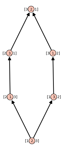
The TransitiveIdeal allows to generates all permutations from the identity permutation using the method permutohedron_succ as successor function:
sage: succ = attrcall("permutohedron_succ")
sage: seed = [Permutation([1,2,3])]
sage: T = TransitiveIdeal(succ, seed)
sage: list(T)
[[1, 2, 3], [2, 1, 3], [1, 3, 2], [2, 3, 1], [3, 2, 1], [3, 1, 2]]
Remark that the previous ordering is neither breadth first neither depth first. It is a naive search because it stores the element to process in a set instead of a queue or a stack.
Note that the method permutohedron_succ produces a graded poset. Therefore, one may use the TransitiveIdealGraded class instead:
sage: T = TransitiveIdealGraded(succ, seed)
sage: list(T)
[[1, 2, 3], [2, 1, 3], [1, 3, 2], [2, 3, 1], [3, 1, 2], [3, 2, 1]]
For TransitiveIdealGraded, the enumeration is breadth first search. Althougth, if you look at the code (version Sage 6.1.1 or earlier), we see that this iterator do not make use of the graded hypothesis at all because the known set remembers every generated elements:
current_level = self._generators
known = set(current_level)
depth = 0
while len(current_level) > 0 and depth <= self._max_depth:
    next_level = set()
    for x in current_level:
        yield x
        for y in self._succ(x):
            if y == None or y in known:
                continue
            next_level.add(y)
            known.add(y)
    current_level = next_level
    depth += 1
return
Timings for TransitiveIdeal
sage: succ = attrcall("permutohedron_succ")
sage: seed = [Permutation([1..5])]
sage: T = TransitiveIdeal(succ, seed)
sage: %time L = list(T)
CPU times: user 26.6 ms, sys: 1.57 ms, total: 28.2 ms
Wall time: 28.5 ms
sage: seed = [Permutation([1..8])]
sage: T = TransitiveIdeal(succ, seed)
sage: %time L = list(T)
CPU times: user 14.4 s, sys: 141 ms, total: 14.5 s
Wall time: 14.8 s
Timings for TransitiveIdealGraded
sage: seed = [Permutation([1..5])]
sage: T = TransitiveIdealGraded(succ, seed)
sage: %time L = list(T)
CPU times: user 25.3 ms, sys: 1.04 ms, total: 26.4 ms
Wall time: 27.4 ms
sage: seed = [Permutation([1..8])]
sage: T = TransitiveIdealGraded(succ, seed)
sage: %time L = list(T)
CPU times: user 14.5 s, sys: 85.8 ms, total: 14.5 s
Wall time: 14.7 s
In conlusion, use TransitiveIdeal for naive search algorithm and use TransitiveIdealGraded for breadth search algorithm. Both class do not use the graded hypothesis.
Recursively enumerated set with a graded structure
The new class RecursivelyEnumeratedSet provides all iterators for each case. The example below are for the graded case.
Depth first search iterator:
sage: succ = attrcall("permutohedron_succ")
sage: seed = [Permutation([1..5])]
sage: R = RecursivelyEnumeratedSet(seed, succ, structure='graded')
sage: it_depth = R.depth_first_search_iterator()
sage: [next(it_depth) for _ in range(5)]
[[1, 2, 3, 4, 5],
 [1, 2, 3, 5, 4],
 [1, 2, 5, 3, 4],
 [1, 2, 5, 4, 3],
 [1, 5, 2, 4, 3]]
Breadth first search iterator:
sage: it_breadth = R.breadth_first_search_iterator()
sage: [next(it_breadth) for _ in range(5)]
[[1, 2, 3, 4, 5],
 [1, 3, 2, 4, 5],
 [1, 2, 4, 3, 5],
 [2, 1, 3, 4, 5],
 [1, 2, 3, 5, 4]]
Elements of given depth iterator:
sage: list(R.elements_of_depth_iterator(9))
[[5, 4, 2, 3, 1], [4, 5, 3, 2, 1], [5, 3, 4, 2, 1], [5, 4, 3, 1, 2]]
sage: list(R.elements_of_depth_iterator(10))
[[5, 4, 3, 2, 1]]
Levels (a level is a set of elements of the same depth):
sage: R.level(0)
[[1, 2, 3, 4, 5]]
sage: R.level(1)
{[1, 2, 3, 5, 4], [1, 2, 4, 3, 5], [1, 3, 2, 4, 5], [2, 1, 3, 4, 5]}
sage: R.level(2)
{[1, 2, 4, 5, 3],
 [1, 2, 5, 3, 4],
 [1, 3, 2, 5, 4],
 [1, 3, 4, 2, 5],
 [1, 4, 2, 3, 5],
 [2, 1, 3, 5, 4],
 [2, 1, 4, 3, 5],
 [2, 3, 1, 4, 5],
 [3, 1, 2, 4, 5]}
sage: R.level(3)
{[1, 2, 5, 4, 3],
 [1, 3, 4, 5, 2],
 [1, 3, 5, 2, 4],
 [1, 4, 2, 5, 3],
 [1, 4, 3, 2, 5],
 [1, 5, 2, 3, 4],
 [2, 1, 4, 5, 3],
 [2, 1, 5, 3, 4],
 [2, 3, 1, 5, 4],
 [2, 3, 4, 1, 5],
 [2, 4, 1, 3, 5],
 [3, 1, 2, 5, 4],
 [3, 1, 4, 2, 5],
 [3, 2, 1, 4, 5],
 [4, 1, 2, 3, 5]}
sage: R.level(9)
{[4, 5, 3, 2, 1], [5, 3, 4, 2, 1], [5, 4, 2, 3, 1], [5, 4, 3, 1, 2]}
sage: R.level(10)
{[5, 4, 3, 2, 1]}
Recursively enumerated set with a symmetric structure
We construct a recursively enumerated set with symmetric structure and depth first search for default enumeration algorithm:
sage: succ = lambda a: [(a[0]-1,a[1]), (a[0],a[1]-1), (a[0]+1,a[1]), (a[0],a[1]+1)]
sage: seeds = [(0,0)]
sage: C = RecursivelyEnumeratedSet(seeds, succ, structure='symmetric', algorithm='depth')
sage: C
A recursively enumerated set with a symmetric structure (depth first search)
In this case, depth first search is the default algorithm for iteration:
sage: it_depth = iter(C)
sage: [next(it_depth) for _ in range(10)]
[(0, 0), (0, 1), (0, 2), (0, 3), (0, 4), (0, 5), (0, 6), (0, 7), (0, 8), (0, 9)]
Breadth first search. This algorithm makes use of the symmetric structure and remembers only the last two levels:
sage: it_breadth = C.breadth_first_search_iterator()
sage: [next(it_breadth) for _ in range(10)]
[(0, 0), (0, 1), (0, -1), (1, 0), (-1, 0), (-1, 1), (-2, 0), (0, 2), (2, 0), (-1, -1)]
Levels (elements of given depth):
sage: sorted(C.level(0))
[(0, 0)]
sage: sorted(C.level(1))
[(-1, 0), (0, -1), (0, 1), (1, 0)]
sage: sorted(C.level(2))
[(-2, 0), (-1, -1), (-1, 1), (0, -2), (0, 2), (1, -1), (1, 1), (2, 0)]
Timings for RecursivelyEnumeratedSet
We get same timings as for TransitiveIdeal but it uses less memory so it might be able to enumerate bigger sets:
sage: succ = attrcall("permutohedron_succ")
sage: seed = [Permutation([1..5])]
sage: R = RecursivelyEnumeratedSet(seed, succ, structure='graded')
sage: %time L = list(R)
CPU times: user 24.7 ms, sys: 1.33 ms, total: 26.1 ms
Wall time: 26.4 ms
sage: seed = [Permutation([1..8])]
sage: R = RecursivelyEnumeratedSet(seed, succ, structure='graded')
sage: %time L = list(R)
CPU times: user 14.5 s, sys: 70.2 ms, total: 14.5 s
Wall time: 14.6 s
« Previous Page -- Next Page »
Propulsé par Blogofile
S'abonner au Flux RSS
et aux Commentaires.

This work by Sébastien Labbé is licensed under a Creative Commons Attribution-ShareAlike 4.0 International License.