Abelian complexity of the Oldenburger sequence

27 septembre 2014 | Catégories: sage | View Comments

The Oldenburger infinite sequence [O39] \[ K = 1221121221221121122121121221121121221221\ldots \] also known under the name of Kolakoski, is equal to its exponent trajectory. The exponent trajectory \(\Delta\) can be obtained by counting the lengths of blocks of consecutive and equal letters: \[ K = 1^12^21^22^11^12^21^12^21^22^11^22^21^12^11^22^11^12^21^22^11^22^11^12^21^12^21^22^11^12^21^12^11^22^11^22^21^12^21^2\ldots \] The sequence of exponents above gives the exponent trajectory of the Oldenburger sequence: \[ \Delta = 12211212212211211221211212\ldots \] which is equal to the original sequence \(K\). You can define this sequence in Sage:

sage: K = words.KolakoskiWord()
sage: K
word: 1221121221221121122121121221121121221221...
sage: K.delta()          # delta returns the exponent trajectory
word: 1221121221221121122121121221121121221221...

There are a lot of open problem related to basic properties of that sequence. For example, we do not know if that sequence is recurrent, that is, all finite subword or factor (finite block of consecutive letters) always reappear. Also, it is still open to prove whether the density of 1 in that sequence is equal to \(1/2\).

In this blog post, I do some computations on its abelian complexity \(p_{ab}(n)\) defined as the number of distinct abelian vectors of subwords of length \(n\) in the sequence. The abelian vector \(\vec{w}\) of a word \(w\) counts the number of occurences of each letter: \[ w = 12211212212 \quad \mapsto \quad 1^5 2^7 \text{, abelianized} \quad \mapsto \quad \vec{w} = (5, 7) \text{, the abelian vector of } w \]

Here are the abelian vectors of subwords of length 10 and 20 in the prefix of length 100 of the Oldenburger sequence. The functions abelian_vectors and abelian_complexity are not in Sage as of now. Code is available at trac #17058 to be merged in Sage soon:

sage: prefix = words.KolakoskiWord()[:100]
sage: prefix.abelian_vectors(10)
{(4, 6), (5, 5), (6, 4)}
sage: prefix.abelian_vectors(20)
{(8, 12), (9, 11), (10, 10), (11, 9), (12, 8)}

Therefore, the prefix of length 100 has 3 vectors of subwords of length 10 and 5 vectors of subwords of length 20:

sage: p100.abelian_complexity(10)
3
sage: p100.abelian_complexity(20)
5

I import the OldenburgerSequence from my optional spkg because it is faster than the implementation in Sage:

sage: from slabbe import KolakoskiWord as OldenburgerSequence
sage: Olden = OldenburgerSequence()

I count the number of abelian vectors of subwords of length 100 in the prefix of length \(2^{20}\) of the Oldenburger sequence:

sage: prefix = Olden[:2^20]
sage: %time prefix.abelian_vectors(100)
CPU times: user 3.48 s, sys: 66.9 ms, total: 3.54 s
Wall time: 3.56 s
{(47, 53), (48, 52), (49, 51), (50, 50), (51, 49), (52, 48), (53, 47)}

Number of abelian vectors of subwords of length less than 100 in the prefix of length \(2^{20}\) of the Oldenburger sequence:

sage: %time L100 = map(prefix.abelian_complexity, range(100))
CPU times: user 3min 20s, sys: 1.08 s, total: 3min 21s
Wall time: 3min 23s
sage: from collections import Counter
sage: Counter(L100)
Counter({5: 26, 6: 26, 4: 17, 7: 15, 3: 8, 8: 4, 2: 3, 1: 1})

Let's draw that:

sage: labels = ('Length of factors', 'Number of abelian vectors')
sage: title = 'Abelian Complexity of the prefix of length $2^{20}$ of Oldenburger sequence'
sage: list_plot(L100, color='green', plotjoined=True, axes_labels=labels, title=title)

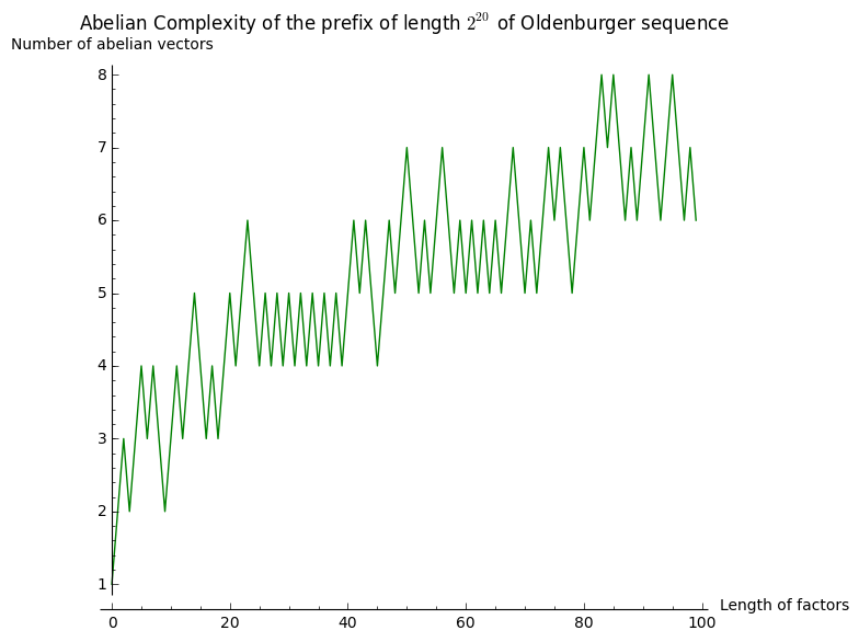
It seems to grow something like \(\log(n)\). Let's now consider subwords of length \(2^n\) for \(0\leq n\leq 12\) in the same prefix of length \(2^{20}\):

sage: %time L20 = [(2^n, prefix.abelian_complexity(2^n)) for n in range(20)]
CPU times: user 41 s, sys: 239 ms, total: 41.2 s
Wall time: 41.5 s
sage: L20
[(1, 2), (2, 3), (4, 3), (8, 3), (16, 3), (32, 5), (64, 5), (128, 9),
(256, 9), (512, 13), (1024, 17), (2048, 22), (4096, 27), (8192, 40),
(16384, 46), (32768, 67), (65536, 81), (131072, 85), (262144, 90), (524288, 104)]

I now look at subwords of length \(2^n\) for \(0\leq n\leq 23\) in the longer prefix of length \(2^{24}\):

sage: prefix = Olden[:2^24]
sage: %time L24 = [(2^n, prefix.abelian_complexity(2^n)) for n in range(24)]
CPU times: user 20min 47s, sys: 13.5 s, total: 21min
Wall time: 20min 13s
sage: L24
[(1, 2), (2, 3), (4, 3), (8, 3), (16, 3), (32, 5), (64, 5), (128, 9), (256,
9), (512, 13), (1024, 17), (2048, 23), (4096, 33), (8192, 46), (16384, 58),
(32768, 74), (65536, 98), (131072, 134), (262144, 165), (524288, 229),
(1048576, 302), (2097152, 371), (4194304, 304), (8388608, 329)]

The next graph gather all of the above computations:

sage: G = Graphics()
sage: legend = 'in the prefix of length 2^{}'
sage: G += list_plot(L24, plotjoined=True, thickness=4, color='blue', legend_label=legend.format(24))
sage: G += list_plot(L20, plotjoined=True, thickness=4, color='red', legend_label=legend.format(20))
sage: G += list_plot(L100, plotjoined=True, thickness=4, color='green', legend_label=legend.format(20))
sage: labels = ('Length of factors', 'Number of abelian vectors')
sage: title = 'Abelian complexity of Oldenburger sequence'
sage: G.show(scale=('semilogx', 2), axes_labels=labels, title=title)

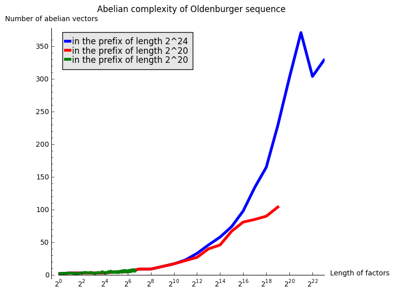
/Files/2014/oldenburger_abelian_2e24.png

A linear growth in the above graphics with logarithmic \(x\) abcisse would mean a growth in \(\log(n)\). After those experimentations, my hypothesis is that the abelian complexity of the Oldenburger sequence grows like \(\log(n)^2\).

References

[O39]

Oldenburger, Rufus (1939). "Exponent trajectories in symbolic dynamics". Transactions of the American Mathematical Society 46: 453–466. doi:10.2307/1989933

Sébastien Labbé

Abelian complexity of the Oldenburger sequence

References