Wooden laser-cut Jeandel-Rao tiles
07 septembre 2018 | Catégories: sage, slabbe spkg, math, découpe laser | View CommentsI have been working on Jeandel-Rao tiles lately.
Before the conference Model Sets and Aperiodic Order held in Durham UK (Sep 3-7 2018), I thought it would be a good idea to bring some real tiles at the conference. So I first decided of some conventions to represent the above tiles as topologically closed disk basically using the representation of integers in base 1:
With these shapes, I created a 33 x 19 patch. With 3cm on each side, the patch takes 99cm x 57cm just within the capacity of the laser cut machine (1m x 60 cm):
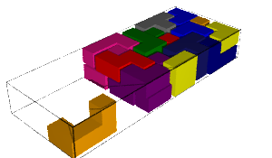
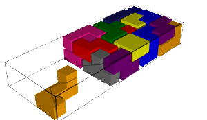
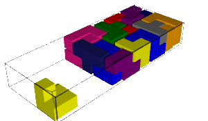
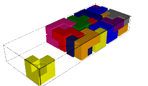
With the help of David Renault from LaBRI, we went at Coh@bit, the FabLab of Bordeaux University and we laser cut two 3mm thick plywood for a total of 1282 Wang tiles. This is the result:
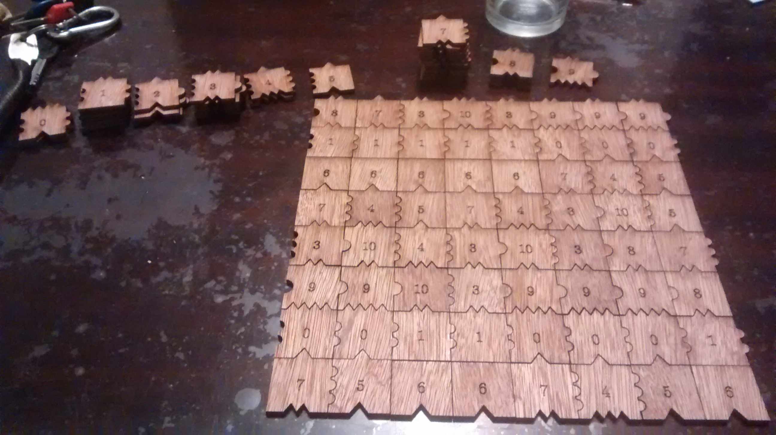
One may recreate the 33 x 19 tiling as follows (note that I am using Cartesian-like coordinates, so the first list data[0] actually is the first column from bottom to top):
sage: data = [[10, 4, 6, 1, 3, 3, 7, 0, 9, 7, 2, 6, 1, 3, 8, 7, 0, 9, 7],
....:  [4, 5, 6, 1, 8, 10, 4, 0, 9, 3, 8, 7, 0, 9, 7, 5, 0, 9, 3],
....:  [3, 7, 6, 1, 7, 2, 5, 0, 9, 8, 7, 5, 0, 9, 3, 7, 0, 9, 10],
....:  [10, 4, 6, 1, 3, 8, 7, 0, 9, 7, 5, 6, 1, 8, 10, 4, 0, 9, 3],
....:  [2, 5, 6, 1, 8, 7, 5, 0, 9, 3, 7, 6, 1, 7, 2, 5, 0, 9, 8],
....:  [8, 7, 6, 1, 7, 5, 6, 1, 8, 10, 4, 6, 1, 3, 8, 7, 0, 9, 7],
....:  [7, 5, 6, 1, 3, 7, 6, 1, 7, 2, 5, 6, 1, 8, 7, 5, 0, 9, 3],
....:  [3, 7, 6, 1, 10, 4, 6, 1, 3, 8, 7, 6, 1, 7, 5, 6, 1, 8, 10],
....:  [10, 4, 6, 1, 3, 3, 7, 0, 9, 7, 5, 6, 1, 3, 7, 6, 1, 7, 2],
....:  [2, 5, 6, 1, 8, 10, 4, 0, 9, 3, 7, 6, 1, 10, 4, 6, 1, 3, 8],
....:  [8, 7, 6, 1, 7, 5, 5, 0, 9, 10, 4, 6, 1, 3, 3, 7, 0, 9, 7],
....:  [7, 5, 6, 1, 3, 7, 6, 1, 10, 4, 5, 6, 1, 8, 10, 4, 0, 9, 3],
....:  [3, 7, 6, 1, 10, 4, 6, 1, 3, 3, 7, 6, 1, 7, 2, 5, 0, 9, 8],
....:  [10, 4, 6, 1, 3, 3, 7, 0, 9, 10, 4, 6, 1, 3, 8, 7, 0, 9, 7],
....:  [4, 5, 6, 1, 8, 10, 4, 0, 9, 3, 3, 7, 0, 9, 7, 5, 0, 9, 3],
....:  [3, 7, 6, 1, 7, 2, 5, 0, 9, 8, 10, 4, 0, 9, 3, 7, 0, 9, 10],
....:  [10, 4, 6, 1, 3, 8, 7, 0, 9, 7, 5, 5, 0, 9, 10, 4, 0, 9, 3],
....:  [2, 5, 6, 1, 8, 7, 5, 0, 9, 3, 7, 6, 1, 10, 4, 5, 0, 9, 8],
....:  [8, 7, 6, 1, 7, 5, 6, 1, 8, 10, 4, 6, 1, 3, 3, 7, 0, 9, 7],
....:  [7, 5, 6, 1, 3, 7, 6, 1, 7, 2, 5, 6, 1, 8, 10, 4, 0, 9, 3],
....:  [3, 7, 6, 1, 10, 4, 6, 1, 3, 8, 7, 6, 1, 7, 2, 5, 0, 9, 8],
....:  [10, 4, 6, 1, 3, 3, 7, 0, 9, 7, 2, 6, 1, 3, 8, 7, 0, 9, 7],
....:  [4, 5, 6, 1, 8, 10, 4, 0, 9, 3, 8, 7, 0, 9, 7, 5, 0, 9, 3],
....:  [3, 7, 6, 1, 7, 2, 5, 0, 9, 8, 7, 5, 0, 9, 3, 7, 0, 9, 10],
....:  [10, 4, 6, 1, 3, 8, 7, 0, 9, 7, 5, 6, 1, 8, 10, 4, 0, 9, 3],
....:  [3, 3, 7, 0, 9, 7, 5, 0, 9, 3, 7, 6, 1, 7, 2, 5, 0, 9, 8],
....:  [8, 10, 4, 0, 9, 3, 7, 0, 9, 10, 4, 6, 1, 3, 8, 7, 0, 9, 7],
....:  [7, 5, 5, 0, 9, 10, 4, 0, 9, 3, 3, 7, 0, 9, 7, 5, 0, 9, 3],
....:  [3, 7, 6, 1, 10, 4, 5, 0, 9, 8, 10, 4, 0, 9, 3, 7, 0, 9, 10],
....:  [10, 4, 6, 1, 3, 3, 7, 0, 9, 7, 5, 5, 0, 9, 10, 4, 0, 9, 3],
....:  [2, 5, 6, 1, 8, 10, 4, 0, 9, 3, 7, 6, 1, 10, 4, 5, 0, 9, 8],
....:  [8, 7, 6, 1, 7, 5, 5, 0, 9, 10, 4, 6, 1, 3, 3, 7, 0, 9, 7],
....:  [7, 5, 6, 1, 3, 7, 6, 1, 10, 4, 5, 6, 1, 8, 10, 4, 0, 9, 3]]
The above patch have been chosen among 1000 other randomly generated as the closest to the asymptotic frequencies of the tiles in Jeandel-Rao tilings (or at least in the minimal subshift that I describe in the preprint):
sage: from collections import Counter
sage: c = Counter(flatten(data))
sage: tile_count = [c[i] for i in range(11)]
The asymptotic frequencies:
sage: phi = golden_ratio.n()
sage: Linv = [2*phi + 6, 2*phi + 6, 18*phi + 10, 2*phi + 6, 8*phi + 2,
....:      5*phi + 4, 2*phi + 6, 12/5*phi + 14/5, 8*phi + 2,
....:      2*phi + 6, 8*phi + 2]
sage: perfect_proportions = vector([1/a for a in Linv])
Comparison of the number of tiles of each type with the expected frequency:
sage: header_row = ['tile id', 'Asymptotic frequency', 'Expected nb of copies',
....:               'Nb copies in the 33x19 patch']
sage: columns = [range(11), perfect_proportions, vector(perfect_proportions)*33*19, tile_count]
sage: table(columns=columns, header_row=header_row)
  tile id   Asymptotic frequency   Expected nb of copies   Nb copies in the 33x19 patch
+---------+----------------------+-----------------------+------------------------------+
  0         0.108271182329550      67.8860313206280        67
  1         0.108271182329550      67.8860313206280        65
  2         0.0255593590340479     16.0257181143480        16
  3         0.108271182329550      67.8860313206280        71
  4         0.0669152706817991     41.9558747174880        42
  5         0.0827118232955023     51.8603132062800        51
  6         0.108271182329550      67.8860313206280        65
  7         0.149627093977301      93.8161879237680        95
  8         0.0669152706817991     41.9558747174880        44
  9         0.108271182329550      67.8860313206280        67
  10        0.0669152706817991     41.9558747174880        44
I brought the \(33\times19=641\) tiles at the conference and offered to the first 7 persons to find a \(7\times 7\) tiling the opportunity to keep the 49 tiles they used. 49 is a good number since the frequency of the lowest tile (with id 2) is about 2% which allows to have at least one copy of each tile in a subset of 49 tiles allowing a solution.
A natural question to ask is how many such \(7\times 7\) tilings does there exist? With ticket #25125 that was merged in Sage 8.3 this Spring, it is possible to enumerate and count solutions in parallel with Knuth dancing links algorithm. After the installation of the Sage Optional package slabbe (sage -pip install slabbe), one may compute that there are 152244 solutions.
sage: from slabbe import WangTileSet
sage: tiles = [(2,4,2,1), (2,2,2,0), (1,1,3,1), (1,2,3,2), (3,1,3,3),
....: (0,1,3,1), (0,0,0,1), (3,1,0,2), (0,2,1,2), (1,2,1,4), (3,3,1,2)]
sage: T0 = WangTileSet(tiles)
sage: T0_solver = T0.solver(7,7)
sage: %time T0_solver.number_of_solutions(ncpus=8)
CPU times: user 16 ms, sys: 82.3 ms, total: 98.3 ms
Wall time: 388 ms
152244
One may also get the list of all solutions and print one of them:
sage: %time L = T0_solver.all_solutions(); print(len(L))
152244
CPU times: user 6.46 s, sys: 344 ms, total: 6.8 s
Wall time: 6.82 s
sage: L[0]
A wang tiling of a 7 x 7 rectangle
sage: L[0].table()  # warning: the output is in Cartesian-like coordinates
[[1, 8, 10, 4, 5, 0, 9],
 [1, 7, 2, 5, 6, 1, 8],
 [1, 3, 8, 7, 6, 1, 7],
 [0, 9, 7, 5, 6, 1, 3],
 [0, 9, 3, 7, 6, 1, 8],
 [1, 8, 10, 4, 6, 1, 7],
 [1, 7, 2, 2, 6, 1, 3]]
This is the number of distinct sets of 49 tiles which admits a 7x7 solution:
sage: from collections import Counter
sage: def count_tiles(tiling):
....:     C = Counter(flatten(tiling.table()))
....:     return tuple(C.get(a,0) for a in range(11))
sage: Lfreq = map(count_tiles, L)
sage: Lfreq_count = Counter(Lfreq)
sage: len(Lfreq_count)
83258
Number of other solutions with the same set of 49 tiles:
sage: Counter(Lfreq_count.values())
Counter({1: 49076, 2: 19849, 3: 6313, 4: 3664, 6: 1410, 5: 1341, 7: 705, 8:
293, 9: 159, 14: 116, 10: 104, 12: 97, 18: 44, 11: 26, 15: 24, 13: 10, 17: 8,
22: 6, 32: 6, 16: 3, 28: 2, 19: 1, 21: 1})
How the number of \(k\times k\)-solutions grows for k from 0 to 9:
sage: [T0.solver(k,k).number_of_solutions() for k in range(10)]
[0, 11, 85, 444, 1723, 9172, 50638, 152244, 262019, 1641695]
Unfortunately, most of those \(k\times k\)-solutions are not extendable to a tiling of the whole plane. Indeed the number of \(k\times k\) patches in the language of the minimal aperiodic subshift that I am able to describe and which is a proper subset of Jeandel-Rao tilings seems, according to some heuristic, to be something like:
[1, 11, 49, 108, 184, 268, 367, 483]
I do not share my (ugly) code for this computation yet, as I will rather share clean code soon when times come. So among the 152244 about only 483 (0.32%) of them are prolongable into a uniformly recurrent tiling of the plane.
A time evolution picture of packages built in parallel by Sage
16 décembre 2016 | Catégories: sage | View CommentsCompiling sage takes a while and does a lot of stuff. Each time I am wondering which components takes so much time and which are fast. I wrote a module in my slabbe version 0.3b2 package available on PyPI to figure this out.
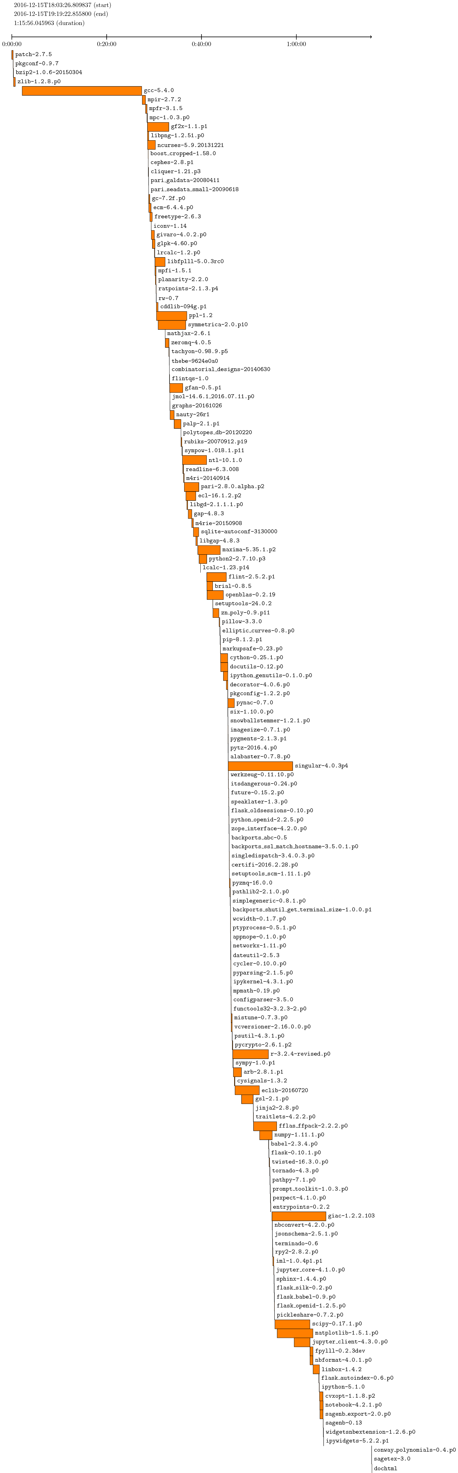
This is after compiling 7.5.beta6 after an upgrade from 7.5.beta4:
sage: from slabbe.analyze_sage_build import draw_sage_build
sage: draw_sage_build().pdf()
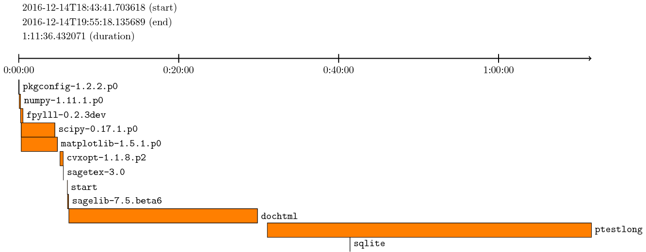
From scratch from a fresh git clone of 7.5.beta6, after running MAKE='make -j4' make ptestlong, I get:
sage: from slabbe.analyze_sage_build import draw_sage_build
sage: draw_sage_build().pdf()
The picture does not include the start and ptestlong because there was an error compiling the documentation.
By default, draw_sage_build considers all of the logs files in logs/pkgs but options are available to consider only log files created in a given interval of time. See draw_sage_build? for more info.
unsupported operand parent for *, Matrix over number field, vector over symbolic ring
18 février 2016 | Catégories: sage | View CommentsYesterday I received this email (in french):
Salut,
avec Thomas on a une question bête:

K.<x>=NumberField(x*x-x-1)

J'aimerais multiplier une matrice avec des coefficients en x par un vecteur
contenant des variables a et b.  Il dit "unsupported operand parent for *,
Matrix over number field, vector over symbolic ring"

Est ce grave ?
Here is my answer. Indeed, in Sage, symbolic variables can't multiply with elements in an Number Field in x:
sage: x = var('x')
sage: K.<x> = NumberField(x*x-x-1)
sage: a = var('a')
sage: a*x
Traceback (most recent call last)
...
TypeError: unsupported operand parent(s) for '*': 'Symbolic Ring' and
'Number Field in x with defining polynomial x^2 - x - 1'
But, we can define a polynomial ring with variables in a,b and coefficients in the NumberField. Then, we are able to multiply a with x:
sage: x = var('x')
sage: K.<x> = NumberField(x*x-x-1)
sage: K
Number Field in x with defining polynomial x^2 - x - 1
sage: R.<a,b> = K['a','b']
sage: R
Multivariate Polynomial Ring in a, b over Number Field in x with
defining polynomial x^2 - x - 1
sage: a*x
(x)*a
With two square brackets, we obtain powers series:
sage: R.<a,b> = K[['a','b']]
sage: R
Multivariate Power Series Ring in a, b over Number Field in x with
defining polynomial x^2 - x - 1
sage: a*x*b
(x)*a*b
It works with matrices:
sage: MS = MatrixSpace(R,2,2)
sage: MS
Full MatrixSpace of 2 by 2 dense matrices over Multivariate Power
Series Ring in a, b over Number Field in x with defining polynomial
x^2 - x - 1
sage: MS([0,a,b,x])
[  0   a]
[  b (x)]
sage: m1 = MS([0,a,b,x])
sage: m2 = MS([0,a+x,b*b+x,x*x])
sage: m1 + m2 * m1
[              (x)*b + a*b       (x + 1) + (x + 1)*a]
[                (x + 2)*b (3*x + 1) + (x)*a + a*b^2]
slabbe-0.2.spkg released
30 novembre 2015 | Catégories: sage, slabbe spkg | View CommentsThese is a summary of the functionalities present in slabbe-0.2.spkg optional Sage package. It works on version 6.8 of Sage but will work best with sage-6.10 (it is using the new code for cartesian_product merged the the betas of sage-6.10). It contains 7 new modules:
- finite_word.py
- language.py
- lyapunov.py
- matrix_cocycle.py
- mult_cont_frac.pyx
- ranking_scale.py
- tikz_picture.py
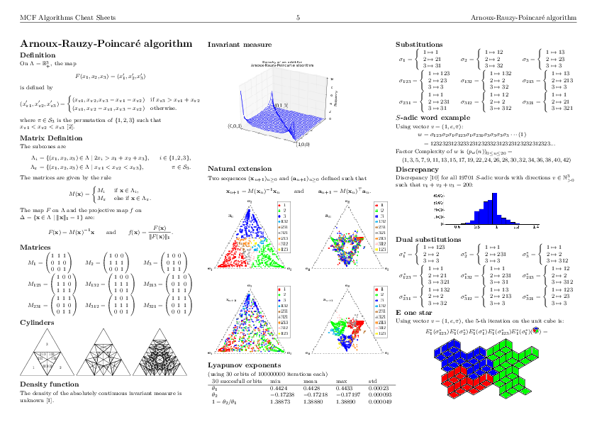
Cheat Sheets
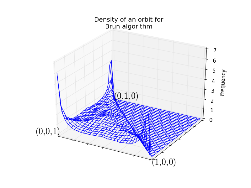
The best way to have a quick look at what can be computed with the optional Sage package slabbe-0.2.spkg is to look at the 3-dimensional Continued Fraction Algorithms Cheat Sheets available on the arXiv since today. It gathers a handful of informations on different 3-dimensional Continued Fraction Algorithms including well-known and old ones (Poincaré, Brun, Selmer, Fully Subtractive) and new ones (Arnoux-Rauzy-Poincaré, Reverse, Cassaigne).
Installation
sage -i http://www.slabbe.org/Sage/slabbe-0.2.spkg    # on sage 6.8
sage -p http://www.slabbe.org/Sage/slabbe-0.2.spkg    # on sage 6.9 or beyond
Examples
Computing the orbit of Brun algorithm on some input in \(\mathbb{R}^3_+\) including dual coordinates:
sage: from slabbe.mult_cont_frac import Brun
sage: algo = Brun()
sage: algo.cone_orbit_list((100, 87, 15), 4)
[(13.0, 87.0, 15.0, 1.0, 2.0, 1.0, 321),
 (13.0, 72.0, 15.0, 1.0, 2.0, 3.0, 132),
 (13.0, 57.0, 15.0, 1.0, 2.0, 5.0, 132),
 (13.0, 42.0, 15.0, 1.0, 2.0, 7.0, 132)]
Computing the invariant measure:
sage: fig = algo.invariant_measure_wireframe_plot(n_iterations=10^6, ndivs=30)
sage: fig.savefig('a.png')
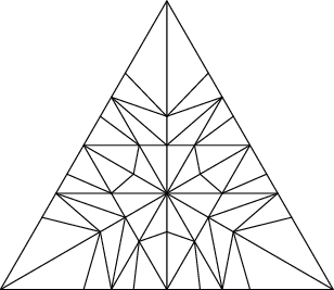
Drawing the cylinders:
sage: cocycle = algo.matrix_cocycle()
sage: t = cocycle.tikz_n_cylinders(3, scale=3)
sage: t.png()
Computing the Lyapunov exponents of the 3-dimensional Brun algorithm:
sage: from slabbe.lyapunov import lyapunov_table
sage: lyapunov_table(algo, n_orbits=30, n_iterations=10^7)
  30 succesful orbits     min       mean      max       std
+-----------------------+---------+---------+---------+---------+
  $\theta_1$              0.3026    0.3045    0.3051    0.00046
  $\theta_2$              -0.1125   -0.1122   -0.1115   0.00020
  $1-\theta_2/\theta_1$   1.3680    1.3684    1.3689    0.00024
Dealing with tikzpictures
Since I create lots of tikzpictures in my code and also because I was unhappy at how the view command of Sage handles them (a tikzpicture is not a math expression to put inside dollar signs), I decided to create a class for tikzpictures. I think this module could be useful in Sage so I will propose its inclusion soon.
I am using the standalone document class which allows some configurations like the border:
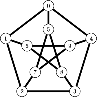
sage: from slabbe import TikzPicture
sage: g = graphs.PetersenGraph()
sage: s = latex(g)
sage: t = TikzPicture(s, standalone_configs=["border=4mm"], packages=['tkz-graph'])
The repr method does not print all of the string since it is often very long. Though it shows how many lines are not printed:
sage: t
\documentclass[tikz]{standalone}
\standaloneconfig{border=4mm}
\usepackage{tkz-graph}
\begin{document}
\begin{tikzpicture}
%
\useasboundingbox (0,0) rectangle (5.0cm,5.0cm);
%
\definecolor{cv0}{rgb}{0.0,0.0,0.0}
...
... 68 lines not printed (3748 characters in total) ...
...
\Edge[lw=0.1cm,style={color=cv6v8,},](v6)(v8)
\Edge[lw=0.1cm,style={color=cv6v9,},](v6)(v9)
\Edge[lw=0.1cm,style={color=cv7v9,},](v7)(v9)
%
\end{tikzpicture}
\end{document}
There is a method to generates a pdf and another for generating a png. Both opens the file in a viewer by default unless view=False:
sage: pathtofile = t.png(density=60, view=False)
sage: pathtofile = t.pdf()
Compare this with the output of view(s, tightpage=True) which does not allow to control the border and also creates a second empty page on some operating system (osx, only one page on ubuntu):
sage: view(s, tightpage=True)
One can also provide the filename where to save the file in which case the file is not open in a viewer:
sage: _ = t.pdf('petersen_graph.pdf')
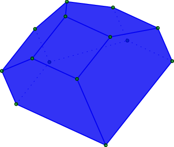
Another example with polyhedron code taken from this Sage thematic tutorial Draw polytopes in LateX using TikZ:
sage: V = [[1,0,1],[1,0,0],[1,1,0],[0,0,-1],[0,1,0],[-1,0,0],[0,1,1],[0,0,1],[0,-1,0]]
sage: P = Polyhedron(vertices=V).polar()
sage: s = P.projection().tikz([674,108,-731],112)
sage: t = TikzPicture(s)
sage: t
\documentclass[tikz]{standalone}
\begin{document}
\begin{tikzpicture}%
        [x={(0.249656cm, -0.577639cm)},
        y={(0.777700cm, -0.358578cm)},
        z={(-0.576936cm, -0.733318cm)},
        scale=2.000000,
...
... 80 lines not printed (4889 characters in total) ...
...
\node[vertex] at (1.00000, 1.00000, -1.00000)     {};
\node[vertex] at (1.00000, 1.00000, 1.00000)     {};
%%
%%
\end{tikzpicture}
\end{document}
sage: _ = t.pdf()
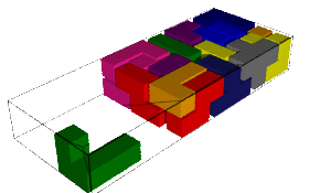
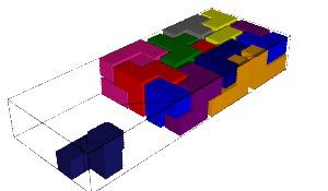
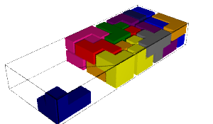
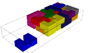
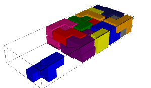
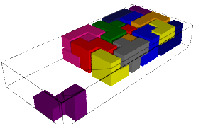
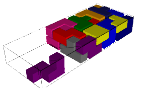
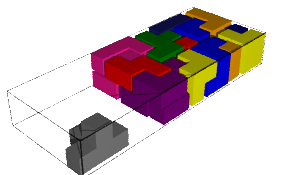
There are 13.366.431.646 solutions to the Quantumino game
21 septembre 2015 | Catégories: sage | View CommentsSome years ago, I wrote code in Sage to solve the Quantumino puzzle. I also used it to make a one-minute video illustrating the Dancing links algorithm which I am proud to say it is now part of the Dancing links wikipedia page.
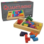
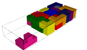
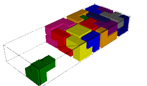
Let me recall that the goal of the Quantumino puzzle is to fill a \(2\times 5\times 8\) box with 16 out of 17 three-dimensional pentaminos. After writing the sage code to solve the puzzle, one question was left: how many solutions are there? Is the official website realist or very prudent when they say that there are over 10.000 potential solutions? Can it be computed in hours? days? months? years? The only thing I knew was that the following computation (letting the 0-th pentamino aside) never finished on my machine:
sage: from sage.games.quantumino import QuantuminoSolver
sage: QuantuminoSolver(0).number_of_solutions()   # long time :)
Since I spent already too much time on this side-project, I decided in 2012 to stop investing any more time on it and to really focus on finishing writing my thesis.
So before I finish writing my thesis, I knew that the computation was not going to take a light-year, since I was able to finish the computation of the number of solutions when the 0-th pentamino is put aside and when one pentamino is pre-positioned somewhere in the box. That computation completed in 4 hours on my old laptop and gave about 5 millions solutions. There are 17 choices of pentatminos to put aside, there are 360 distinct positions of that pentamino in the box, so I estimated the number of solution to be something like \(17\times 360\times 5000000 = 30 \times 10^9\). Most importantly, I estimated the computation to take \(17\times 360\times 4= 24480\) hours or 1020 days. Therefore, I knew I could not do it on my laptop.
But last year, I received an email from the designer of the Quantumino puzzle:
-------- Message transféré --------
Sujet : quantumino
Date : Tue, 09 Dec 2014 13:22:30 +0100
De : Nicolaas Neuwahl
Pour : Sebastien Labbe

hi sébastien labbé,

i'm the designer of the quantumino puzzle.
i'm not a mathematician, i'm an architect. i like mathematics.
i'm quite impressed to see the sage work on quantumino, also i have not the
knowledge for full understanding.

i have a question for you - can you tell me HOW MANY different quantumino-
solutions exist?

ty and bye

nicolaas neuwahl
This summer was a good timing to launch the computation on my beautiful Intel® Core™ i5-4590 CPU @ 3.30GHz × 4 at Université de Liège. First, I improved the Sage code to allow a parallel computation of number of solutions in the dancing links code (#18987, merged in a Sage 6.9.beta6). Secondly, we may remark that each tiling of the \(2\times 5\times 8\) box can be rotated in order to find 3 other solutions. It is possible to gain a factor 4 by avoiding to count 4 times the same solution up to rotations (#19107, still needs work from myself). Thanks to Vincent Delecroix for doing the review on both ticket. Dividing the estimated 1024 days of computation needed by a factor \(4\times 4=16\) gives an approximation of 64 days to complete the computation. Two months, just enough to be tractable!
With those two tickets (some previous version to be honest) on top of sage-6.8, I started the computation on August 4th and the computation finished last week on September 18th for a total of 45 days. The computation was stopped only once on September 8th (I forgot to close firefox and thunderbird that night...).
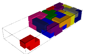
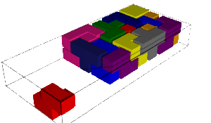
The number of solutions and computation time for each pentamino put aside together with the first solution found is shown in the table below. We remark that some values are equal when the aside pentaminoes are miror images (why!?:).
|
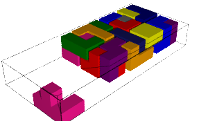
|
| 634 900 493 solutions | 634 900 493 solutions |
| 2 days, 6:22:44.883358 | 2 days, 6:19:08.945691 |
|
|
| 509 560 697 solutions | 509 560 697 solutions |
| 2 days, 0:01:36.844612 | 2 days, 0:41:59.447773 |
|
|
| 628 384 422 solutions | 628 384 422 solutions |
| 2 days, 7:52:31.459247 | 2 days, 8:44:49.465672 |
|
|
| 1 212 362 145 solutions | 1 212 362 145 solutions |
| 3 days, 17:25:00.346627 | 3 days, 19:10:02.353063 |
|
|
| 197 325 298 solutions | 556 534 800 solutions |
| 22:51:54.439932 | 1 day, 19:05:23.908326 |
|
|
| 664 820 756 solutions | 468 206 736 solutions |
| 2 days, 8:48:54.767662 | 1 day, 20:14:56.014557 |
|
|
| 1 385 955 043 solutions | 1 385 955 043 solutions |
| 4 days, 1:40:30.270929 | 4 days, 4:44:05.399367 |
|
|
| 694 998 374 solutions | 694 998 374 solutions |
| 2 days, 11:44:29.631 | 2 days, 6:01:57.946708 |
|
|
| 1 347 221 708 solutions | |
| 3 days, 21:51:29.043459 |
Therefore the total number of solutions up to rotations is 13 366 431 646 which is indeed more than 10000:)
sage: L = [634900493, 634900493, 509560697, 509560697, 628384422,
628384422, 1212362145, 1212362145, 197325298, 556534800, 664820756,
468206736, 1385955043, 1385955043, 694998374, 694998374, 1347221708]
sage: sum(L)
13366431646
sage: factor(_)
2 * 23 * 271 * 1072231
| The machine (4 cores) | Intel® Core™ i5-4590 CPU @ 3.30GHz × 4 (Université de Liège) |
| Computation Time | 45 days, (Aug 4th -- Sep 18th, 2015) |
| Number of solutions (up to rotations) | 13 366 431 646 |
| Number of solutions / cpu / second | 859 |
My code will be available on github.
About the video on wikipedia.
I must say that the video is not perfect. On wikipedia, the file talk page of the video says that the Jerky camera movement is distracting. That is because I managed to make the video out of images created by .show(viewer='tachyon') which changes the coordinate system, hardcodes a lot of parameters, zoom properly, simplifies stuff to make sure the user don't see just a blank image. But, for making a movie, we need access to more parameters especially the placement of the camera (to avoid the jerky movement). I know that Tachyon allows all of that. It is still a project that I have to create a more versatile Graphics3D -> Tachyon conversion allowing to construct nice videos of evolving mathematical objects. That's another story.
« Previous Page -- Next Page »
Propulsé par Blogofile
S'abonner au Flux RSS
et aux Commentaires.

This work by Sébastien Labbé is licensed under a Creative Commons Attribution-ShareAlike 4.0 International License.