La version finale de ma thèse de doctorat intitulée Structure des pavages, droites discrètes 3D et combinatoire des mots est maintenant disponible dans la section Publications. Les diapositives de la soutenance le sont aussi dans la section Communications. La soutenance a eu lieu le 4 mai 2012 à l'Université du Québec à Montréal et des photos sont sur le site du LaCIM.

Existe-t-il des méthodes pour calculer l'inverse d'une matrice rectangulaire non carrée. Je me souviens qu'Ernest Monga nous avait fait travailler sur ce sujet dans un cours qu'il donnait à l'Université de Sherbrooke. Il a notamment donné une présentation Inverse généralisé d’une matrice quelconque – application à deux problèmes statistiques au camp 2011 de l'AMQ.

À l'aide de quelques conditions, il est possible de définir l'inverse d'une matrice rectangulaire de façon unique. Plus d'informations sont disponibles dans le livre Probabilités, analyse des données et statistique sur books.google.ca, sur Wikipédia Pseudo-inverse. Sur la page de wikipédia en anglais Moore-Penrose pseudoinverse, on trouve aussi une section Software libraries mentionnant que les librairies NumPy et SciPy peuvent calculer cette matrice pseudo-inverse.

sage: m = matrix(2, range(6))
sage: m
[0 1 2]
[3 4 5]
sage: mm = numpy.matrix(m)
sage: mm
matrix([[0, 1, 2],
        [3, 4, 5]])
sage: mm.I
matrix([[-0.77777778,  0.27777778],
        [-0.11111111,  0.11111111],
        [ 0.55555556, -0.05555556]])
sage: mm * mm.I
matrix([[  1.00000000e+00,  -1.38777878e-16],
        [  3.10862447e-15,   1.00000000e+00]])
sage: mm.I * mm
matrix([[ 0.83333333,  0.33333333, -0.16666667],
        [ 0.33333333,  0.33333333,  0.33333333],
        [-0.16666667,  0.33333333,  0.83333333]])

Alors que la fonction Moore-Penrose Matrix Inverse est présente dans Mathematica, je crois qu'elle n'est pas encore présente dans Sage sans passer par NumPy. Peut-être qu'une implémentation basée sur l'article Fast Computation of Moore-Penrose Inverse Matrices de Pierre Courrieu (2008) pourrait être effectuée.

Voici le préambule latex que j'utilise souvent:

\documentclass[12pt]{article}

\usepackage{amsmath}
\usepackage{amsfonts}
\usepackage{latexsym}
\usepackage{graphicx}
\usepackage{amssymb}
\usepackage{amsthm}
\usepackage[margin=2cm]{geometry}
\usepackage{url}
\usepackage{color}
\usepackage{enumerate}
\usepackage[shortlabels]{enumitem} %pour commencer les enumerations a des nombres differents
\usepackage[small]{caption}
\usepackage{cite}

Pour des fichiers en français, j'utilise les packages suivants:

\usepackage[T1]{fontenc}     % Hyphénation des mots accentués
\usepackage{lmodern}         % Polices vectorielles

\usepackage[french]{babel}   % Vocabulaire en francais
\usepackage[utf8]{inputenc}  % Codage UNICODE (UTF-8)

Doron Zeilbeger made a talk last Friday at CRM in Montreal during Sage Days 38 about \(n^{n-2}\). At the end of the talk, he propoed a contest to code Joyal's Bijection which relates double rooted trees on \(n\) vertices and endofunctions on \(n\) elements. I wrote an implementation in Sage. My code is available here : joyal_bijection.sage. It will certainly not win for the most brief code, but it is object oriented, documented, reusable, testable and allows introspection.

sage: load joyal_bijection.sage

sage: L = [7, 0, 6, 1, 4, 7, 2, 1, 5]
sage: f = Endofunction(L)
sage: f
Endofunction:
[0..8] -> [7, 0, 6, 1, 4, 7, 2, 1, 5]

sage: L = [(0,6),(2,1),(3,1),(4,2),(5,7),(6,4),(7,0),(8,5)]
sage: D = DoubleRootedTree(L, 1, 7)
sage: D
Double rooted tree:
Edges: [(0, 6), (2, 1), (3, 1), (4, 2), (5, 7), (6, 4), (7, 0), (8, 5)]
RootA: 1
RootB: 7

sage: f.to_double_rooted_tree()
Double rooted tree:
Edges: [(0, 6), (2, 1), (3, 1), (4, 2), (5, 7), (6, 4), (7, 0), (8, 5)]
RootA: 1
RootB: 7

sage: D.to_endofunction()
Endofunction:
[0..8] -> [7, 0, 6, 1, 4, 7, 2, 1, 5]

sage: D == f.to_double_rooted_tree()
True
sage: f == D.to_endofunction()
True

sage: E = Endofunctions(10000)
sage: f = E.random_element()
sage: time f == f.to_double_rooted_tree().to_endofunction()
True
Time: CPU 2.23 s, Wall: 2.24 s

On December 21 2011, version 0.12 of IPython was released with its own notebook. The differences with the Sage Notebook are explained by Fernando Perez, leader of IPython project, in the blog post The IPython notebook: a historical retrospective he wrote last January. One of the differences is that the IPython Notebook run in its own directory whereas each cell of the Sage Notebook lives in its directory.

The latest version of IPython is 0.12.1 and was released in April 2012 and I was curious of testing it. I followed the installations informations. I got into trouble some times but finally managed to install it. Below is how I did to install IPython 0.12.1 on my OSX 10.5.8 using Python 2.6.7.

Installing dependencies:

sudo easy_install-2.6 tornado
sudo easy_install-2.6 nose
sudo easy_install-2.6 pyzmq

The following command was broken for a while:

sudo easy_install-2.6 pyzmq

ending with error TypeError: 'NoneType' object is not callable. I managed to make it work by redoing the above install commands in the correct above order:

sudo easy_install-2.6 tornado
sudo easy_install-2.6 nose
sudo easy_install-2.6 pyzmq

Installing ipython-0.12:

sudo easy_install-2.6 ipython

To make ipython known from the command line, I added the following line to the file ~/.bash_profile:

# ipython
export PATH=/opt/local/Library/Frameworks/Python.framework/Versions/2.6/bin:$PATH

I tested the ipython installation with the iptest command. It finishes with Status: OK

iptest

I open the ipython notebook and it worked:

ipython notebook
[NotebookApp] Using existing profile dir: u'/Users/slabbe/.ipython/profile_default'
[NotebookApp] The IPython Notebook is running at: http://127.0.0.1:8888
[NotebookApp] Use Control-C to stop this server and shut down all kernels.

In safari, I get the following problem:

Websocket connection to
ws://127.0.0.1:8888/kernels/86fef706-f386-4116-b3e4-d6d7776afb0d could not
be established.  You will NOT be able to run code.  Your browser may not be
compatible with the websocket version in the server, or if the url does not
look right, there could be an error in the server's configuration.

But, in firefox, it works when I open a page at the above adress http://127.0.0.1:8888. It gives me the following dashboard page.

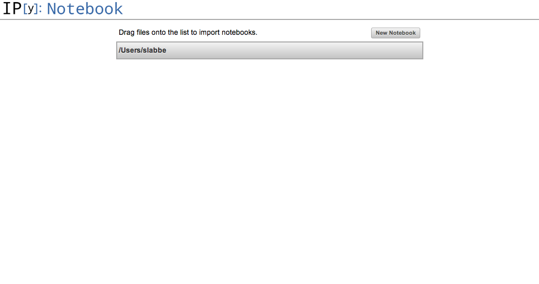
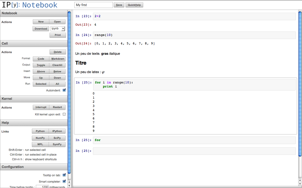
I created my first notebook and did some tests. I followed the documentation found here.

The next thing would be to try to use this with Sage. Some progress has been done and can be followed at ticket #12719.