Installation de Python, Jupyter et JupyterLab
23 février 2021 | Catégories: sage, math | View CommentsL'École doctorale de mathématiques et informatique (EDMI) de l'Université de Bordeaux offre des cours chaque année. Dans ce cadre, cette année, je donnerai le cours Calcul et programmation avec Python ou SageMath et meilleures pratiques qui aura lieu les 25 février, 4 mars, 11 mars, 18 mars 2021 de 9h à 12h.
Le créneau du jeudi matin correspond au créneau des Jeudis Sage au LaBRI où un groupe d'utilisateurs de Python se rencontrent toutes les semaines pour faire du développement tout en posant des questions aux autres utilisateurs présents.
Le cours aura lieu sur le logiciel BigBlueButton auquel les participantEs inscritEs se connecteront par leur navigateur web (Mozilla Firefox ou Google Chrome). Selon les exigences minimales du client BigBlueButton, il faut éviter Safari ou IE, sinon certaines fonctionnalités ne marchent pas. Vous pouvez vous familiariser avec l'interface BigBlueButton en écoutant ce tutoriel BigBlueButton (sur youtube, 5 minutes). Consultez les pages de support suivantes en cas de soucis audio ou internet.
Pour la première séance, nous présenterons les bases de Python et les différentes interfaces. Nous ne pourrons pas passer trop de temps à faire l'installation des différents logiciels. Il serait donc préférable si les installations ont déjà été faites avant le cours par chacun des participantEs. Cela vous permettra de reproduire les commandes montrées et faire des exercices.
Les logiciels à installer avant le cours sont:
- Python3
- SageMath (facultatif)
- IPython
- Jupyter notebook classique
- JupyterLab
Python 3: Normalement, Python est déjà installé sur votre ordinateur. Vous pouvez le confirmer en tapant python ou python3 dans un terminal (Linux/Mac) ou dans l'invité de commande (Windows). Vous devriez obtenir quelque chose qui ressemble à ceci:
Python 3.8.5 (default, Jul 28 2020, 12:59:40)
[GCC 9.3.0] on linux
Type "help", "copyright", "credits" or "license" for more information.
>>>
SageMath (facultatif): SageMath est un logiciel libre de mathématiques basé sur Python et regroupant des centaines de packages et librairies. Il y a plusieurs manières d'installer SageMath, et je vous recommande de lire cette documentation pour déterminer la manière de l'installer qui vous convient le mieux. Sinon, vous pouvez télécharger directement les binaires ici.
Vous devriez obtenir quelque chose qui ressemble à ceci:
┌────────────────────────────────────────────────────────────────────┐
│ SageMath version 9.2, Release Date: 2020-10-24                     │
│ Using Python 3.8.5. Type "help()" for help.                        │
└────────────────────────────────────────────────────────────────────┘
sage:
IPython:
Si vous avez déjà installé SageMath, c'est bon, car ipython en fait partie. La commande sage -ipython vous permettra de l'ouvrir.
Si vous n'avez pas SageMath, vous pouvez l'installer via pip install ipython ou sinon en suivant ces instructions du site ipython. Ensuite, la commande ipython dans le terminal (Linux, OS X) ou dans l'invité de commande (Windows) vous permettra de l'ouvrir.
Vous devriez obtenir quelque chose qui ressemble à ceci:
Python 3.8.5 (default, Jul 28 2020, 12:59:40)
Type 'copyright', 'credits' or 'license' for more information
IPython 7.13.0 -- An enhanced Interactive Python. Type '?' for help.

In [1]:
Jupyter:
Si vous avez déjà installé SageMath, c'est bon, car Jupyter en fait partie. La commande sage -n jupyter vous permettra de l'ouvrir.
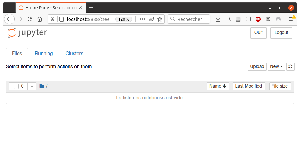
Si vous n'avez pas SageMath, vous pouvez suivre ces instructions du site jupyter.org. Ensuite, la commande jupyter notebook dans le terminal (Linux, OS X) ou dans l'invité de commande (Windows) vous permettra de l'ouvrir.
Vous devriez obtenir quelque chose qui ressemble à ceci dans votre navigateur:
JupyterLab:
Si vous avez déjà installé SageMath, vous pouvez installer JupyterLab en faisant sage -i jupyterlab et l'ouvrir en faisant sage -n jupyterlab. Sur Windows, c'est un tout petit peut différent, il faut plutôt faire pip install jupyterlab dans la console SageMath selon cette récente réponse sur ask.sagemath.org.
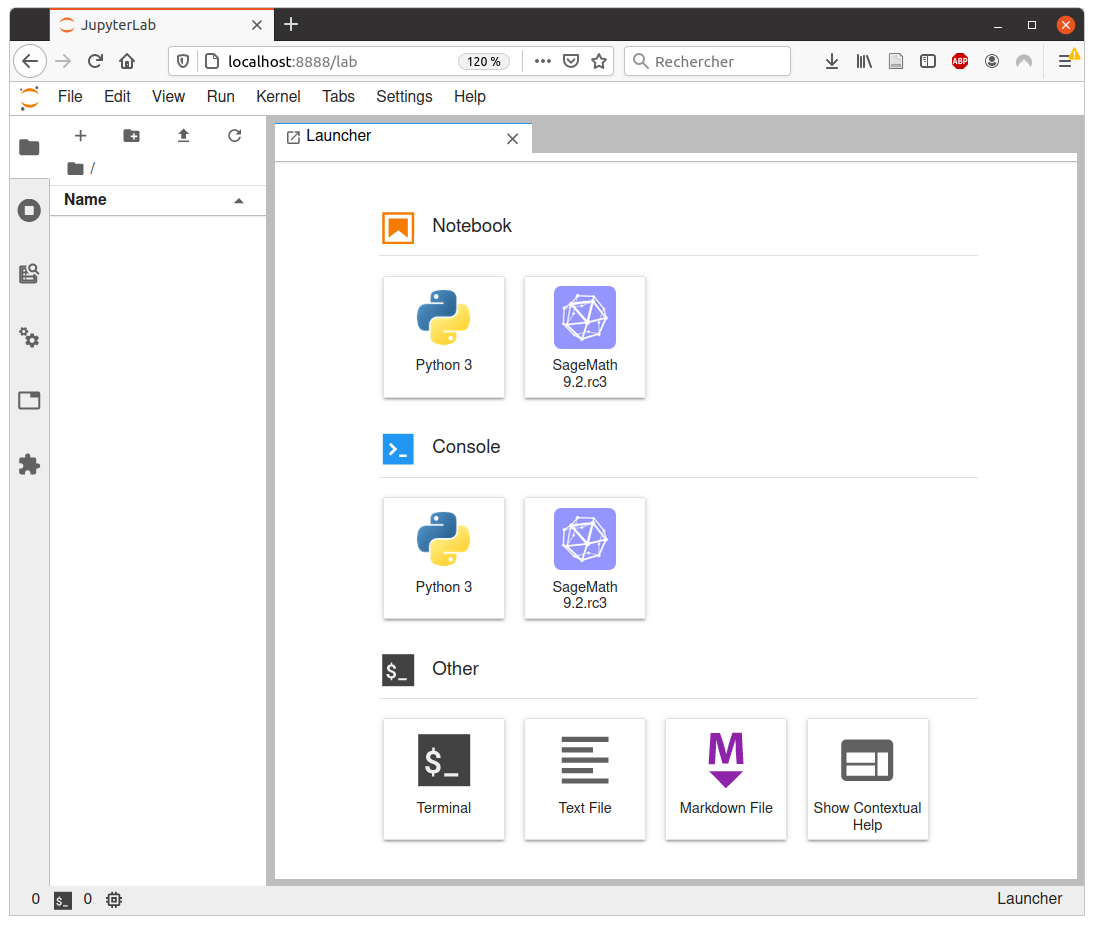
Si vous n'avez pas SageMath, vous pouvez suivre les instructions du même site que ci-haut. Ensuite, la commande jupyter-lab ou jupyter lab dans le terminal (Linux, OS X) ou dans l'invité de commande (Windows) vous permettra de l'ouvrir.
Vous devriez obtenir quelque chose qui ressemble à ceci dans votre navigateur:
Tiling a polyomino with polyominoes in SageMath
03 décembre 2020 | Catégories: sage, math | View CommentsSuppose that you 3D print many copies of the following 3D hexo-mino at home:
sage: from sage.combinat.tiling import Polyomino, TilingSolver
sage: p = Polyomino([(0,0,0), (0,1,0), (1,0,0), (2,0,0), (2,1,0), (2,1,1)], color='blue')
sage: p.show3d()
Launched html viewer for Graphics3d Object
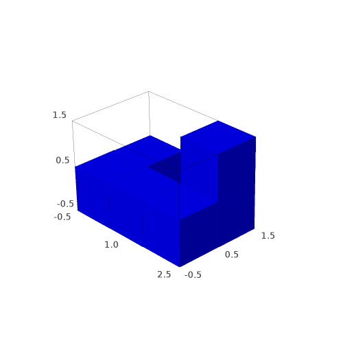
You would like to know if you can tile a larger polyomino or in particular a rectangular box with many copies of it. The TilingSolver module in SageMath is made for that. See also this recent question on ask.sagemath.org.
sage: T = TilingSolver([p], (7,5,3), rotation=True, reflection=False, reusable=True)
sage: T
Tiling solver of 1 pieces into a box of size 24
Rotation allowed: True
Reflection allowed: False
Reusing pieces allowed: True
There is no solution when tiling a box of shape 7x5x3 with this polyomino:
sage: T.number_of_solutions()
0
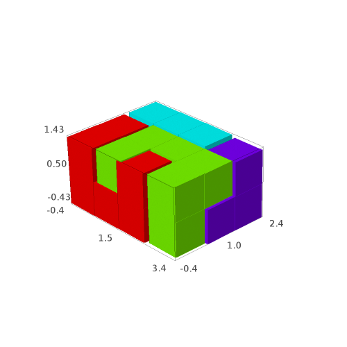
But there are 4 solutions when tiling a box of shape 4x3x2 with this polyomino:
sage: T = TilingSolver([p], (4,3,2), rotation=True, reflection=False, reusable=True)
sage: T.number_of_solutions()
4
We construct the list of solutions:
sage: solutions = [sol for sol in T.solve()]
Each solution contains the isometric copies of the polyominoes tiling the box:
sage: solutions[0]
[Polyomino: [(0, 0, 0), (0, 0, 1), (0, 1, 0), (1, 1, 0), (2, 0, 0), (2, 1, 0)], Color: #ff0000,
 Polyomino: [(0, 1, 1), (0, 2, 0), (0, 2, 1), (1, 1, 1), (2, 1, 1), (2, 2, 1)], Color: #ff0000,
 Polyomino: [(1, 0, 0), (1, 0, 1), (2, 0, 1), (3, 0, 0), (3, 0, 1), (3, 1, 0)], Color: #ff0000,
 Polyomino: [(1, 2, 0), (1, 2, 1), (2, 2, 0), (3, 1, 1), (3, 2, 0), (3, 2, 1)], Color: #ff0000]
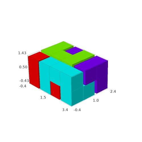
It may be easier to visualize the solutions, so we define the following function allowing to draw the solutions with different colors for each piece:
sage: def draw_solution(solution, size=0.9):
....:     colors = rainbow(len(solution))
....:     for piece,col in zip(solution, colors):
....:         piece.color(col)
....:     return sum((piece.show3d(size=size) for piece in solution), Graphics())
sage: G = [draw_solution(sol) for sol in solutions]
sage: G
[Graphics3d Object, Graphics3d Object, Graphics3d Object, Graphics3d Object]
sage: G[0] # in Sage, this will open a 3d viewer automatically
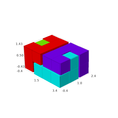
sage: G[1]
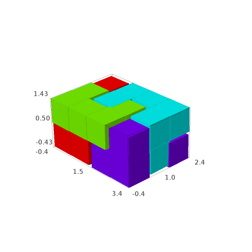
sage: G[2]
sage: G[3]
We may save the solutions to a file:
sage: G[0].save('solution0.png', aspect_ratio=1, zoom=1.2)
sage: G[1].save('solution1.png', aspect_ratio=1, zoom=1.2)
sage: G[2].save('solution2.png', aspect_ratio=1, zoom=1.2)
sage: G[3].save('solution3.png', aspect_ratio=1, zoom=1.2)
Question: are all of the 4 solutions isometric to each other?
The tiling problem is solved due to a reduction to the exact cover problem for which dancing links Knuth's algorithm provides all the solutions. One can see the rows of the dancing links matrix as follows:
sage: d = T.dlx_solver()
sage: d
Dancing links solver for 24 columns and 56 rows
sage: d.rows()
[[0, 1, 2, 4, 5, 11],
 [6, 7, 8, 10, 11, 17],
 [12, 13, 14, 16, 17, 23],
 ...
 [4, 6, 7, 9, 10, 11],
 [10, 12, 13, 15, 16, 17],
 [16, 18, 19, 21, 22, 23]]
The solutions to the dlx solver can be obtained as follows:
sage: it = d.solutions_iterator()
sage: next(it)
[3, 36, 19, 52]
These are the indices of the rows each corresponding to an isometric copy of the polyomino within the box.
Since SageMath-9.2, the possibility to reduce the problem to a MILP problem or a SAT instance was added to SageMath (see #29338 and #29955):
sage: d.to_milp()
(Boolean Program (no objective, 56 variables, 24 constraints),
 MIPVariable of dimension 1)
sage: d.to_sat_solver()
CryptoMiniSat solver: 56 variables, 2348 clauses.
Computer experiments for the Lyapunov exponent for MCF algorithms when dimension is larger than 3
27 mars 2020 | Catégories: sage, slabbe spkg, math | View CommentsIn November 2015, I wanted to share intuitions I developped on the behavior of various distinct Multidimensional Continued Fractions algorithms obtained from various kind of experiments performed with them often involving combinatorics and digitial geometry but also including the computation of their first two Lyapunov exponents.
As continued fractions are deeply related to the combinatorics of Sturmian sequences which can be seen as the digitalization of a straight line in the grid \(\mathbb{Z}^2\), the multidimensional continued fractions algorithm are related to the digitalization of a straight line and hyperplanes in \(\mathbb{Z}^d\).
This is why I shared those experiments in what I called 3-dimensional Continued Fraction Algorithms Cheat Sheets because of its format inspired from typical cheat sheets found on the web. All of the experiments can be reproduced using the optional SageMath package slabbe where I share my research code. People asked me whether I was going to try to publish those Cheat Sheets, but I was afraid the format would change the organization of the information and data in each page, so, in the end, I never submitted those Cheat Sheets anywhere.
Here I should say that \(d\) stands for the dimension of the vector space on which the involved matrices act and \(d-1\) is the dimension of the projective space on which the algorithm acts.
One of the consequence of the Cheat Sheets is that it made us realize that the algorithm proposed by Julien Cassaigne had the same first two Lyapunov exponents as the Selmer algorithm (first 3 significant digits were the same). Julien then discovered the explanation as its algorithm is conjugated to some semi-sorted version of the Selmer algorihm. This result was shared during WORDS 2017 conference. Julien Leroy, Julien Cassaigne and I are still working on the extended version of the paper. It is taking longer mainly because of my fault because I have been working hard on aperiodic Wang tilings in the previous 2 years.
During July 2019, Wolfgang, Valérie and Jörg asked me to perform computations of the first two Lyapunov exponents for \(d\)-dimensional Multidimensional Continued Fraction algorithms for \(d\) larger than 3. The main question of interest is whether the second Lyapunov exponent keeps being negative as the dimension increases. This property is related to the notion of strong convergence almost everywhere of the simultaneous diopantine approximations provided by the algorithm of a fixed vector of real numbers. It did not take me too long to update my package since I had started to generalize my code to larger dimensions during Fall 2017. It turns out that, as the dimension increases, all known MCF algorithms have their second Lyapunov exponent become positive. My computations were thus confirming what they eventually published in their preprint in November 2019.
My motivation for sharing the results is the conference Multidimensional Continued Fractions and Euclidean Dynamics held this week (supposed to be held in Lorentz Center, March 23-27 2020, it got cancelled because of the corona virus) where some discussions during video meetings are related to this subject.
The computations performed below can be summarized in one graphics showing the values of \(1-\theta_2/\theta_1\) with respect to \(d\) for various \(d\)-dimensional MCF algorithms. It seems that \(\theta_2\) is negative up to dimension 10 for Brun, up to dimension 4 for Selmer and up to dimension 5 for ARP.
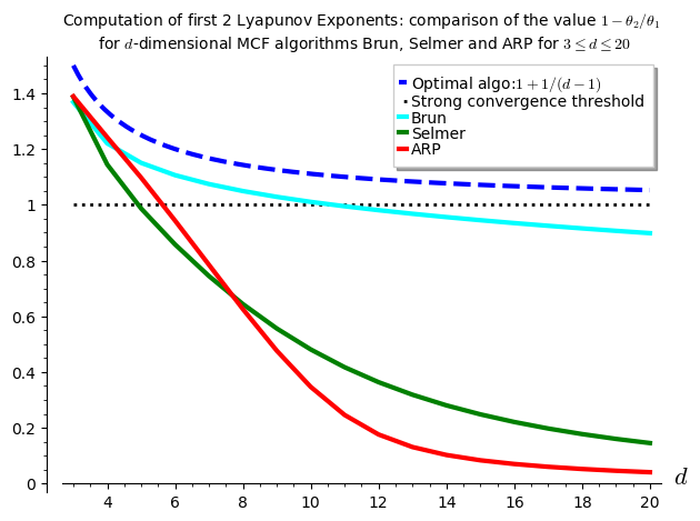
I have to say that I was disapointed by the results because the algorithm Arnoux-Rauzy-Poincaré (ARP) that Valérie and I introduced was not performing so well as its second Lyapunov exponent seems to become positive for dimension \(d\geq 6\). I had good expectations for ARP because it reaches the highest value for \(1-\theta_2/\theta_1\) in the computations performed in the Cheat Sheets, thus better than Brun, better than Selmer when \(d=3\).
The algorithm for the computation of the first two Lyapunov exponents was provided to me by Vincent Delecroix. It applies the algorithm \((v,w)\mapsto(M^{-1}v,M^T w)\) millions of times. The evolution of the size of the vector \(v\) gives the first Lyapunov exponent. The evolution of the size of the vector \(w\) gives the second Lyapunov exponent. Since the computation is performed on 64-bits double floating point number, their are numerical issues to deal with. This is why some Gramm Shimdts operation is performed on the vector \(w\) at each time the vectors are renormalized to keep the vector \(w\) orthogonal to \(v\). Otherwise, the numerical errors cumulate and the computed value for the \(\theta_2\) becomes the same as \(\theta_1\). You can look at the algorithm online starting at line 1723 of the file mult_cont_frac_pyx.pyx from my optional package.
I do not know from where Vincent took that algorithm. So, I do not know how exact it is and whether there exits any proof of lower bounds and upper bounds on the computations being performed. What I can say is that it is quite reliable in the sense that is returns the same values over and over again (by that I mean 3 common most significant digits) with any fixed inputs (number of iterations).
Below, I show the code illustrating how to reproduce the results.
The version 0.6 (November 2019) of my package slabbe includes the necessary code to deal with some \(d\)-dimensional Multidimensional Continued Fraction (MCF) algorithms. Its documentation is available online. It is a PIP package, so it can be installed like this:
sage -pip install slabbe
Recall that the dimension \(d\) below is the linear one and \(d-1\) is the dimension of the space for the corresponding projective algorithm.
Import the Brun, Selmer and Arnoux-Rauzy-Poincaré MCF algorithms from the optional package:
sage: from slabbe.mult_cont_frac import Brun, Selmer, ARP
The computation of the first two Lyapunov exponents performed on one single orbit:
sage: Brun(dim=3).lyapunov_exponents(n_iterations=10^7)
(0.30473782969922547, -0.11220958022368056, 1.3682167728713919)
The starting point is taken randomly, but the results of the form of a 3-tuple \((\theta_1,\theta_2,1-\theta_2/\theta_1)\) are about the same:
sage: Brun(dim=3).lyapunov_exponents(n_iterations=10^7)
(0.30345018206132324, -0.11171509867725296, 1.3681497170915415)
Increasing the dimension \(d\) yields:
sage: Brun(dim=4).lyapunov_exponents(n_iterations=10^7)
(0.32639514522732005, -0.07191456560115839, 1.2203297648654456)
sage: Brun(dim=5).lyapunov_exponents(n_iterations=10^7)
(0.30918877340506756, -0.0463930802132972, 1.1500477514185734)
It performs an orbit of length \(10^7\) in about .5 seconds, of length \(10^8\) in about 5 seconds and of length \(10^9\) in about 50 seconds:
sage: %time Brun(dim=3).lyapunov_exponents(n_iterations=10^7)
CPU times: user 540 ms, sys: 0 ns, total: 540 ms
Wall time: 539 ms
(0.30488799356325225, -0.11234354880132114, 1.3684748208296182)
sage: %time Brun(dim=3).lyapunov_exponents(n_iterations=10^8)
CPU times: user 5.09 s, sys: 0 ns, total: 5.09 s
Wall time: 5.08 s
(0.30455473631148755, -0.11217550411862384, 1.3683262505689446)
sage: %time Brun(dim=3).lyapunov_exponents(n_iterations=10^9)
CPU times: user 51.2 s, sys: 0 ns, total: 51.2 s
Wall time: 51.2 s
(0.30438755982577026, -0.11211562816821799, 1.368331834035505)
Here, in what follows, I must admit that I needed to do a small fix to my package, so the code below will not work in version 0.6 of my package, I will update my package in the next days in order that the computations below can be reproduced:
sage: from slabbe.lyapunov import lyapunov_comparison_table
For each \(3\leq d\leq 20\), I compute 30 orbits and I show the most significant digits and the standard deviation of the 30 values computed.
For Brun algorithm:
sage: algos = [Brun(d) for d in range(3,21)]
sage: %time lyapunov_comparison_table(algos, n_orbits=30, n_iterations=10^7, ncpus=8)
CPU times: user 190 ms, sys: 2.8 s, total: 2.99 s
Wall time: 6min 31s
  Algorithm     \#Orbits   $\theta_1$ (std)     $\theta_2$ (std)      $1-\theta_2/\theta_1$ (std)
+-------------+----------+--------------------+---------------------+-----------------------------+
  Brun (d=3)    30         0.3045 (0.00040)     -0.1122 (0.00017)     1.3683 (0.00022)
  Brun (d=4)    30         0.32632 (0.000055)   -0.07188 (0.000051)   1.2203 (0.00014)
  Brun (d=5)    30         0.30919 (0.000032)   -0.04647 (0.000041)   1.1503 (0.00013)
  Brun (d=6)    30         0.28626 (0.000027)   -0.03043 (0.000035)   1.1063 (0.00012)
  Brun (d=7)    30         0.26441 (0.000024)   -0.01966 (0.000027)   1.0743 (0.00010)
  Brun (d=8)    30         0.24504 (0.000027)   -0.01207 (0.000024)   1.04926 (0.000096)
  Brun (d=9)    30         0.22824 (0.000021)   -0.00649 (0.000026)   1.0284 (0.00012)
  Brun (d=10)   30         0.2138 (0.00098)     -0.0022 (0.00015)     1.0104 (0.00074)
  Brun (d=11)   30         0.20085 (0.000015)   0.00106 (0.000022)    0.9947 (0.00011)
  Brun (d=12)   30         0.18962 (0.000017)   0.00368 (0.000021)    0.9806 (0.00011)
  Brun (d=13)   30         0.17967 (0.000011)   0.00580 (0.000020)    0.9677 (0.00011)
  Brun (d=14)   30         0.17077 (0.000011)   0.00755 (0.000021)    0.9558 (0.00012)
  Brun (d=15)   30         0.16278 (0.000012)   0.00900 (0.000017)    0.9447 (0.00010)
  Brun (d=16)   30         0.15556 (0.000011)   0.01022 (0.000013)    0.93433 (0.000086)
  Brun (d=17)   30         0.149002 (9.5e-6)    0.01124 (0.000015)    0.9246 (0.00010)
  Brun (d=18)   30         0.14303 (0.000010)   0.01211 (0.000019)    0.9153 (0.00014)
  Brun (d=19)   30         0.13755 (0.000012)   0.01285 (0.000018)    0.9065 (0.00013)
  Brun (d=20)   30         0.13251 (0.000011)   0.01349 (0.000019)    0.8982 (0.00014)
For Selmer algorithm:
sage: algos = [Selmer(d) for d in range(3,21)]
sage: %time lyapunov_comparison_table(algos, n_orbits=30, n_iterations=10^7, ncpus=8)
CPU times: user 203 ms, sys: 2.78 s, total: 2.98 s
Wall time: 6min 27s
  Algorithm       \#Orbits   $\theta_1$ (std)     $\theta_2$ (std)      $1-\theta_2/\theta_1$ (std)
+---------------+----------+--------------------+---------------------+-----------------------------+
  Selmer (d=3)    30         0.1827 (0.00041)     -0.0707 (0.00017)     1.3871 (0.00029)
  Selmer (d=4)    30         0.15808 (0.000058)   -0.02282 (0.000036)   1.1444 (0.00023)
  Selmer (d=5)    30         0.13199 (0.000033)   0.00176 (0.000034)    0.9866 (0.00026)
  Selmer (d=6)    30         0.11205 (0.000017)   0.01595 (0.000036)    0.8577 (0.00031)
  Selmer (d=7)    30         0.09697 (0.000012)   0.02481 (0.000030)    0.7442 (0.00032)
  Selmer (d=8)    30         0.085340 (8.5e-6)    0.03041 (0.000032)    0.6437 (0.00036)
  Selmer (d=9)    30         0.076136 (5.9e-6)    0.03379 (0.000032)    0.5561 (0.00041)
  Selmer (d=10)   30         0.068690 (5.5e-6)    0.03565 (0.000023)    0.4810 (0.00032)
  Selmer (d=11)   30         0.062557 (4.4e-6)    0.03646 (0.000021)    0.4172 (0.00031)
  Selmer (d=12)   30         0.057417 (3.6e-6)    0.03654 (0.000017)    0.3636 (0.00028)
  Selmer (d=13)   30         0.05305 (0.000011)   0.03615 (0.000018)    0.3186 (0.00032)
  Selmer (d=14)   30         0.04928 (0.000060)   0.03546 (0.000051)    0.2804 (0.00040)
  Selmer (d=15)   30         0.046040 (2.0e-6)    0.03462 (0.000013)    0.2482 (0.00027)
  Selmer (d=16)   30         0.04318 (0.000011)   0.03365 (0.000014)    0.2208 (0.00028)
  Selmer (d=17)   30         0.040658 (3.3e-6)    0.03263 (0.000013)    0.1974 (0.00030)
  Selmer (d=18)   30         0.038411 (2.7e-6)    0.031596 (9.8e-6)     0.1774 (0.00022)
  Selmer (d=19)   30         0.036399 (2.2e-6)    0.030571 (8.0e-6)     0.1601 (0.00019)
  Selmer (d=20)   30         0.0346 (0.00011)     0.02955 (0.000093)    0.1452 (0.00019)
For Arnoux-Rauzy-Poincaré algorithm:
sage: algos = [ARP(d) for d in range(3,21)]
sage: %time lyapunov_comparison_table(algos, n_orbits=30, n_iterations=10^7, ncpus=8)
CPU times: user 226 ms, sys: 2.76 s, total: 2.99 s
Wall time: 13min 20s
  Algorithm                        \#Orbits   $\theta_1$ (std)     $\theta_2$ (std)      $1-\theta_2/\theta_1$ (std)
+--------------------------------+----------+--------------------+---------------------+-----------------------------+
  Arnoux-Rauzy-Poincar\'e (d=3)    30         0.4428 (0.00056)     -0.1722 (0.00025)     1.3888 (0.00016)
  Arnoux-Rauzy-Poincar\'e (d=4)    30         0.6811 (0.00020)     -0.16480 (0.000085)   1.24198 (0.000093)
  Arnoux-Rauzy-Poincar\'e (d=5)    30         0.7982 (0.00012)     -0.0776 (0.00010)     1.0972 (0.00013)
  Arnoux-Rauzy-Poincar\'e (d=6)    30         0.83563 (0.000091)   0.0475 (0.00010)      0.9432 (0.00012)
  Arnoux-Rauzy-Poincar\'e (d=7)    30         0.8363 (0.00011)     0.1802 (0.00016)      0.7845 (0.00020)
  Arnoux-Rauzy-Poincar\'e (d=8)    30         0.8213 (0.00013)     0.3074 (0.00023)      0.6257 (0.00028)
  Arnoux-Rauzy-Poincar\'e (d=9)    30         0.8030 (0.00012)     0.4205 (0.00017)      0.4763 (0.00022)
  Arnoux-Rauzy-Poincar\'e (d=10)   30         0.7899 (0.00011)     0.5160 (0.00016)      0.3467 (0.00020)
  Arnoux-Rauzy-Poincar\'e (d=11)   30         0.7856 (0.00014)     0.5924 (0.00020)      0.2459 (0.00022)
  Arnoux-Rauzy-Poincar\'e (d=12)   30         0.7883 (0.00010)     0.6497 (0.00012)      0.1759 (0.00014)
  Arnoux-Rauzy-Poincar\'e (d=13)   30         0.7930 (0.00010)     0.6892 (0.00014)      0.1309 (0.00014)
  Arnoux-Rauzy-Poincar\'e (d=14)   30         0.7962 (0.00012)     0.7147 (0.00015)      0.10239 (0.000077)
  Arnoux-Rauzy-Poincar\'e (d=15)   30         0.7974 (0.00012)     0.7309 (0.00014)      0.08340 (0.000074)
  Arnoux-Rauzy-Poincar\'e (d=16)   30         0.7969 (0.00015)     0.7411 (0.00014)      0.07010 (0.000048)
  Arnoux-Rauzy-Poincar\'e (d=17)   30         0.7960 (0.00014)     0.7482 (0.00014)      0.06005 (0.000050)
  Arnoux-Rauzy-Poincar\'e (d=18)   30         0.7952 (0.00013)     0.7537 (0.00014)      0.05218 (0.000046)
  Arnoux-Rauzy-Poincar\'e (d=19)   30         0.7949 (0.00012)     0.7584 (0.00013)      0.04582 (0.000035)
  Arnoux-Rauzy-Poincar\'e (d=20)   30         0.7948 (0.00014)     0.7626 (0.00013)      0.04058 (0.000025)
The computation of the figure shown above is done with the code below:
sage: brun_list = [1.3683, 1.2203, 1.1503, 1.1063, 1.0743, 1.04926, 1.0284, 1.0104, 0.9947, 0.9806, 0.9677, 0.9558, 0.9447, 0.93433, 0.9246, 0.9153, 0.9065, 0.8982]
sage: selmer_list = [ 1.3871, 1.1444, 0.9866, 0.8577, 0.7442, 0.6437, 0.5561, 0.4810, 0.4172, 0.3636, 0.3186, 0.2804, 0.2482, 0.2208, 0.1974, 0.1774, 0.1601, 0.1452]
sage: arp_list = [1.3888, 1.24198, 1.0972, 0.9432, 0.7845, 0.6257, 0.4763, 0.3467, 0.2459, 0.1759, 0.1309, 0.10239, 0.08340, 0.07010, 0.06005, 0.05218, 0.04582, 0.04058]
sage: brun_points = list(enumerate(brun_list, start=3))
sage: selmer_points = list(enumerate(selmer_list, start=3))
sage: arp_points = list(enumerate(arp_list, start=3))
sage: G = Graphics()
sage: G += plot(1+1/(x-1), x, 3, 20, legend_label='Optimal algo:$1+1/(d-1)$', linestyle='dashed', color='blue', thickness=3)
sage: G += line([(3,1), (20,1)], color='black', legend_label='Strong convergence threshold', linestyle='dotted', thickness=2)
sage: G += line(brun_points, legend_label='Brun', color='cyan', thickness=3)
sage: G += line(selmer_points, legend_label='Selmer', color='green', thickness=3)
sage: G += line(arp_points, legend_label='ARP', color='red', thickness=3)
sage: G.ymin(0)
sage: G.axes_labels(['$d$',''])
sage: G.show(title='Computation of first 2 Lyapunov Exponents: comparison of the value $1-\\theta_2/\\theta_1$\n for $d$-dimensional MCF algorithms Brun, Selmer and ARP for $3\\leq d\\leq 20$')
Comment installer et utiliser RISE, une extension du notebook Jupyter pour faire des présentations
24 janvier 2019 | Catégories: sage | View CommentsLa semaine dernière, Jeroen Demeyer a fait une présentation lors de l'Atelier PARI/GP 2019 au sujet de cypari2.
La présentation de Jeroen consistait en des diapositives HTML où les calculs sont faits en direct (avec Jupyter) et où on peut les modifier en direct dans les diapositives. Impressionant! Tout cela grâce au package Python RISE.
Pour installer et utiliser RISE, une extension du Jupyter Notebook pour faire des présentations éditables, il ne suffit pas de l'installer il faut aussi recopier les css au bon endroit. Pour l'installer dans Sage, il suffit de faire:
sage -pip install rise
sage -sh
jupyter-nbextension install rise --py --sys-prefix
Après on peut consulter ce démo sur youtube et la documentation de RISE est ici.
Comparison of Wang tiling solvers
12 décembre 2018 | Catégories: sage, slabbe spkg, math | View CommentsDuring the last year, I have written a Python module to deal with Wang tiles containing about 4K lines of code including doctests and documentation.
It can be installed like this:
sage -pip install slabbe
It can be used like this:
sage: from slabbe import WangTileSet
sage: tiles = [(2,4,2,1), (2,2,2,0), (1,1,3,1), (1,2,3,2), (3,1,3,3),
....: (0,1,3,1), (0,0,0,1), (3,1,0,2), (0,2,1,2), (1,2,1,4), (3,3,1,2)]
sage: T0 = WangTileSet([tuple(str(a) for a in t) for t in tiles])
sage: T0.tikz(ncolumns=11).pdf()
The module on wang tiles contains a class WangTileSolver which contains three reductions of the Wang tiling problem the first using MILP solvers, the second using SAT solvers and the third using Knuth's dancing links.
Here is one example of a tiling found using the dancing links reduction:
sage: %time tiling = T0.solver(10,10).solve(solver='dancing_links')
CPU times: user 36 ms, sys: 12 ms, total: 48 ms
Wall time: 65.5 ms
sage: tiling.tikz().pdf()
All these reductions now allow me to compare the efficiency of various types of solvers restricted to the Wang tiling type of problems. Here is the list of solvers that I often use.
| Solver | Description |
|---|---|
| 'Gurobi' | MILP solver |
| 'GLPK' | MILP solver |
| 'PPL' | MILP solver |
| 'LP' | a SAT solver using a reduction to LP |
| 'cryptominisat' | SAT solver |
| 'picosat' | SAT solver |
| 'glucose' | SAT solver |
| 'dancing_links' | Knuth's algorihm |
In this recent work on the substitutive structure of Jeandel-Rao tilings, I introduced various Wang tile sets \(T_i\) for \(i\in\{0,1,\dots,12\}\). In this blog post, we will concentrate on the 11 Wang tile set \(T_0\) introduced by Jeandel and Rao as well as \(T_2\) containing 20 tiles and \(T_3\) containing 24 tiles.
Tiling a n x n square
The most natural question to ask is to find valid Wang tilings of \(n\times n\) square with given Wang tiles. Below is the time spent by each mentionned solvers to find a valid tiling of a \(n\times n\) square in less than 10 seconds for each of the three wang tile sets \(T_0\), \(T_2\) and \(T_3\).
We remark that MILP solvers are slower. Dancing links can solve 20x20 squares with Jeandel Rao tiles \(T_0\) and SAT solvers are performing very well with Glucose being the best as it can find a 55x55 tiling with Jeandel-Rao tiles \(T_0\) in less than 10 seconds.
Finding all dominoes allowing a surrounding of given radius
One thing that is often needed in my research is to enumerate all horizontal and vertical dominoes that allow a given surrounding radius. This is a difficult question in general as deciding if a given tile set admits a tiling of the infinite plane is undecidable. But in some cases, the information we get from the dominoes admitting a surrounding of radius 1, 2, 3 or 4 is enough to conclude that the tiling can be desubstituted for instance. This is why we need to answer this question as fast as possible.
Below is the comparison in the time taken by each solver to compute all vertical and horizontal dominoes allowing a surrounding of radius 1, 2 and 3 (in less than 1000 seconds for each execution).
What is surprising at first is that the solvers that performed well in the first \(n\times n\) square experience are not the best in the second experiment computing valid dominoes. Dancing links and the MILP solver Gurobi are now the best algorithms to compute all dominoes. They are followed by picosat and cryptominisat and then glucose.
The source code of the above comparisons
The source code of the above comparison can be found in this Jupyter notebook. Note that it depends on the use of Glucose as a Sage optional package (#26361) and on the most recent development version of slabbe optional Sage Package.
« Previous Page -- Next Page »
Propulsé par Blogofile
S'abonner au Flux RSS
et aux Commentaires.

This work by Sébastien Labbé is licensed under a Creative Commons Attribution-ShareAlike 4.0 International License.