À Liège, une piste cyclable dans la trémie parking du pont Kennedy
20 juin 2022 | Catégories: urbanisme | View CommentsJeudi 16 juin 2022, en marchant du centre vers le parc de la Boverie pour le rendez-vous du jeudi soir de la conférence DYADISC, j'ai eu l'agréable surprise de voir que trois des 25 suggestions que j'avais faites en 2016 ont été réalisées:
- Créer une piste cyclable dans la trémie parking du pont Kennedy, afin de désengorger la ravel qui devrait être réservée aux piétons qui marchent le long de la meuse.
- Sur le quai Marcellis, remplacer du stationnement par une piste cyclable qui emprunte la trémie du pont Kennedy, pour la même raison de réserver le ravel aux piétons dans Outremeuse.
- Créer une piste cyclable sur la place Cockerill pour prolonger le flux de vélo qui emprunte la passerelle piétonne devant la Grande Poste.
C'est super!
Using Glucose SAT solver to find a tiling of a rectangle by polyominoes
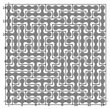
27 mai 2021 | Mise à jour: 20 juin 2022 | Catégories: sage, math | View CommentsIn his Dancing links article, Donald Knuth considered the problem of packing 45 Y pentaminoes into a 15 x 15 square. We can redo this computation in SageMath using some implementation of his dancing links algorithm.
Dancing links takes 1.24 seconds to find a solution:
sage: from sage.combinat.tiling import Polyomino, TilingSolver
sage: y = Polyomino([(0,0),(1,0),(2,0),(3,0),(2,1)])
sage: T = TilingSolver([y], box=(15, 15), reusable=True, reflection=True)
sage: %time solution = next(T.solve())
CPU times: user 1.23 s, sys: 11.9 ms, total: 1.24 s
Wall time: 1.24 s
The first solution found is:
sage: sum(T.row_to_polyomino(row_number).show2d() for row_number in solution)
What is nice about dancing links algorithm is that it can list all solutions to a problem. For example, it takes less than 3 minutes to find all solutions of tiling a 15 x 15 rectangle with the Y polyomino:
sage: %time T.number_of_solutions()
CPU times: user 2min 46s, sys: 3.46 ms, total: 2min 46s
Wall time: 2min 46s
1696
It takes more time (38s) to find a first solution of a larger 20 x 20 rectangle:
sage: T = TilingSolver([y], box=(20,20), reusable=True, reflection=True)
sage: %time solution = next(T.solve())
CPU times: user 38.2 s, sys: 7.88 ms, total: 38.2 s
Wall time: 38.2 s
The polyomino tiling problem is reduced to an instance of the universal cover problem which is represented by a sparse matrix of 0 and 1:
sage: dlx = T.dlx_solver()
sage: dlx
Dancing links solver for 400 columns and 2584 rows
We observe that finding a solution to this problem takes the same amount of time. This is normal since it is exactly what is used behind the scene when calling next(T.solve()) above:
sage: %time sol = dlx.one_solution(ncpus=1)
CPU times: user 38.6 s, sys: 48 ms, total: 38.6 s
Wall time: 38.5 s
One way to improve the time it takes it to split the problem into parts and use many processors to work on each subproblems. Here a random column is used to split the problem which may affect the time it takes. Sometimes a good column is chosen and it works great as below, but sometimes it does not:
sage: %time sol = dlx.one_solution(ncpus=2)
CPU times: user 941 µs, sys: 32 ms, total: 32.9 ms
Wall time: 1.41 s
The reduction from dancing links instance to SAT instance #29338 and to MILP instance #29955 was merged into SageMath 9.2 during the last year. A discussion with Franco Saliola motivated me to implement these translations since he was also searching for faster way to solve dancing links problems. Indeed some problems are solved faster with other kind of solver, so it is good to make some comparisons between solvers.
Therefore, with a recent enough version of SageMath, we can now try to find a tiling with other kinds of solvers. Following my experience with tilings by Wang tiles, I know that Glucose SAT solver is quite efficient to solve tilings of the plane. This is why I test this one below. Glucose is now an optional package to SageMath which can be installed with:
sage -i glucose
Update (June 20th, 2022): It seems sage -i glucose no longer works. The new procedure is to use ./configure --enable-glucose when installation is made from source. See the question Unable to install glucose SAT solver with Sage on ask.sagemath.org for more information.
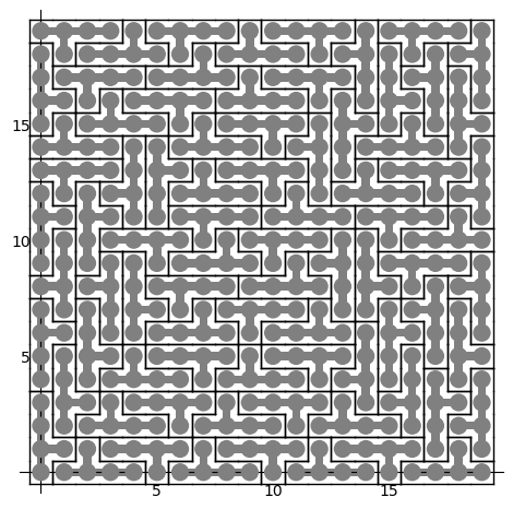
Glucose finds the solution of a 20 x 20 rectangle in 1.5 seconds:
sage: %time sol = dlx.one_solution_using_sat_solver('glucose')
CPU times: user 306 ms, sys: 12.1 ms, total: 319 ms
Wall time: 1.51 s
The rows of the solution found by Glucose are:
sage: sol
[0, 15, 19, 38, 74, 245, 270, 310, 320, 327, 332, 366, 419, 557, 582, 613, 660,
 665, 686, 699, 707, 760, 772, 774, 781, 802, 814, 816, 847, 855, 876, 905,
 1025, 1070, 1081, 1092, 1148, 1165, 1249, 1273, 1283, 1299, 1354, 1516, 1549,
 1599, 1609, 1627, 1633, 1650, 1717, 1728, 1739, 1773, 1795, 1891, 1908, 1918,
 1995, 2004, 2016, 2029, 2037, 2090, 2102, 2104, 2111, 2132, 2144, 2146, 2185,
 2235, 2301, 2460, 2472, 2498, 2538, 2548, 2573, 2583]
Each row correspond to a Y polyomino embedded in the plane in a certain position:
sage: sum(T.row_to_polyomino(row_number).show2d() for row_number in sol)
Glucose-Syrup (a parallelized version of Glucose) takes about the same time (1 second) to find a tiling of a 20 x 20 rectangle:
sage: T = TilingSolver([y], box=(20, 20), reusable=True, reflection=True)
sage: dlx = T.dlx_solver()
sage: dlx
Dancing links solver for 400 columns and 2584 rows
sage: %time sol = dlx.one_solution_using_sat_solver('glucose-syrup')
CPU times: user 285 ms, sys: 20 ms, total: 305 ms
Wall time: 1.09 s
Searching for a tiling of a 30 x 30 rectangle, Glucose takes 40s and Glucose-Syrup takes 16s while dancing links algorithm takes much longer (next(T.solve()) which is using dancing links algorithm does not halt in less than 5 minutes):
sage: T = TilingSolver([y], box=(30,30), reusable=True, reflection=True)
sage: dlx = T.dlx_solver()
sage: dlx
Dancing links solver for 900 columns and 6264 rows
sage: %time sol = dlx.one_solution_using_sat_solver('glucose')
CPU times: user 708 ms, sys: 36 ms, total: 744 ms
Wall time: 40.5 s
sage: %time sol = dlx.one_solution_using_sat_solver('glucose-syrup')
CPU times: user 754 ms, sys: 39.1 ms, total: 793 ms
Wall time: 16.1 s
Searching for a tiling of a 35 x 35 rectangle, Glucose takes 2min 5s and Glucose-Syrup takes 1min 16s:
sage: T = TilingSolver([y], box=(35, 35), reusable=True, reflection=True)
sage: dlx = T.dlx_solver()
sage: dlx
Dancing links solver for 1225 columns and 8704 rows
sage: %time sol = dlx.one_solution_using_sat_solver('glucose')
CPU times: user 1.07 s, sys: 47.9 ms, total: 1.12 s
Wall time: 2min 5s
sage: %time sol = dlx.one_solution_using_sat_solver('glucose-syrup')
CPU times: user 1.06 s, sys: 24 ms, total: 1.09 s
Wall time: 1min 16s
Here are the info of the computer used for the above timings (a 4 years old laptop runing Ubuntu 20.04):
$ lscpu
Architecture :                          x86_64
Mode(s) opératoire(s) des processeurs : 32-bit, 64-bit
Boutisme :                              Little Endian
Address size :                          39 bits physical, 48 bits virtual
Processeur(s) :                         8
Liste de processeur(s) en ligne :       0-7
Thread(s) par coeur :                   2
Coeur(s) par socket :                   4
Socket(s) :                             1
Noeud(s) NUMA :                         1
Identifiant constructeur :              GenuineIntel
Famille de processeur :                 6
Modèle :                                158
Nom de modèle :                         Intel(R) Core(TM) i7-7820HQ CPU @ 2.90GHz
Révision :                              9
Vitesse du processeur en MHz :          3549.025
Vitesse maximale du processeur en MHz : 3900,0000
Vitesse minimale du processeur en MHz : 800,0000
BogoMIPS :                              5799.77
Virtualisation :                        VT-x
Cache L1d :                             128 KiB
Cache L1i :                             128 KiB
Cache L2 :                              1 MiB
Cache L3 :                              8 MiB
Noeud NUMA 0 de processeur(s) :         0-7
To finish, I should mention that the implementation of dancing links made in SageMath is not the best one. Indeed, according to what Franco Saliola told me, the dancing links code written by Donald Knuth himself and available on his website (franco added some makefile to compile it more easily) is faster. It would be interesting to confirm this and if possible improves the implementation made in SageMath.
Installation de Python, Jupyter et JupyterLab
23 février 2021 | Catégories: sage, math | View CommentsL'École doctorale de mathématiques et informatique (EDMI) de l'Université de Bordeaux offre des cours chaque année. Dans ce cadre, cette année, je donnerai le cours Calcul et programmation avec Python ou SageMath et meilleures pratiques qui aura lieu les 25 février, 4 mars, 11 mars, 18 mars 2021 de 9h à 12h.
Le créneau du jeudi matin correspond au créneau des Jeudis Sage au LaBRI où un groupe d'utilisateurs de Python se rencontrent toutes les semaines pour faire du développement tout en posant des questions aux autres utilisateurs présents.
Le cours aura lieu sur le logiciel BigBlueButton auquel les participantEs inscritEs se connecteront par leur navigateur web (Mozilla Firefox ou Google Chrome). Selon les exigences minimales du client BigBlueButton, il faut éviter Safari ou IE, sinon certaines fonctionnalités ne marchent pas. Vous pouvez vous familiariser avec l'interface BigBlueButton en écoutant ce tutoriel BigBlueButton (sur youtube, 5 minutes). Consultez les pages de support suivantes en cas de soucis audio ou internet.
Pour la première séance, nous présenterons les bases de Python et les différentes interfaces. Nous ne pourrons pas passer trop de temps à faire l'installation des différents logiciels. Il serait donc préférable si les installations ont déjà été faites avant le cours par chacun des participantEs. Cela vous permettra de reproduire les commandes montrées et faire des exercices.
Les logiciels à installer avant le cours sont:
- Python3
- SageMath (facultatif)
- IPython
- Jupyter notebook classique
- JupyterLab
Python 3: Normalement, Python est déjà installé sur votre ordinateur. Vous pouvez le confirmer en tapant python ou python3 dans un terminal (Linux/Mac) ou dans l'invité de commande (Windows). Vous devriez obtenir quelque chose qui ressemble à ceci:
Python 3.8.5 (default, Jul 28 2020, 12:59:40)
[GCC 9.3.0] on linux
Type "help", "copyright", "credits" or "license" for more information.
>>>
SageMath (facultatif): SageMath est un logiciel libre de mathématiques basé sur Python et regroupant des centaines de packages et librairies. Il y a plusieurs manières d'installer SageMath, et je vous recommande de lire cette documentation pour déterminer la manière de l'installer qui vous convient le mieux. Sinon, vous pouvez télécharger directement les binaires ici.
Vous devriez obtenir quelque chose qui ressemble à ceci:
┌────────────────────────────────────────────────────────────────────┐
│ SageMath version 9.2, Release Date: 2020-10-24                     │
│ Using Python 3.8.5. Type "help()" for help.                        │
└────────────────────────────────────────────────────────────────────┘
sage:
IPython:
Si vous avez déjà installé SageMath, c'est bon, car ipython en fait partie. La commande sage -ipython vous permettra de l'ouvrir.
Si vous n'avez pas SageMath, vous pouvez l'installer via pip install ipython ou sinon en suivant ces instructions du site ipython. Ensuite, la commande ipython dans le terminal (Linux, OS X) ou dans l'invité de commande (Windows) vous permettra de l'ouvrir.
Vous devriez obtenir quelque chose qui ressemble à ceci:
Python 3.8.5 (default, Jul 28 2020, 12:59:40)
Type 'copyright', 'credits' or 'license' for more information
IPython 7.13.0 -- An enhanced Interactive Python. Type '?' for help.

In [1]:
Jupyter:
Si vous avez déjà installé SageMath, c'est bon, car Jupyter en fait partie. La commande sage -n jupyter vous permettra de l'ouvrir.
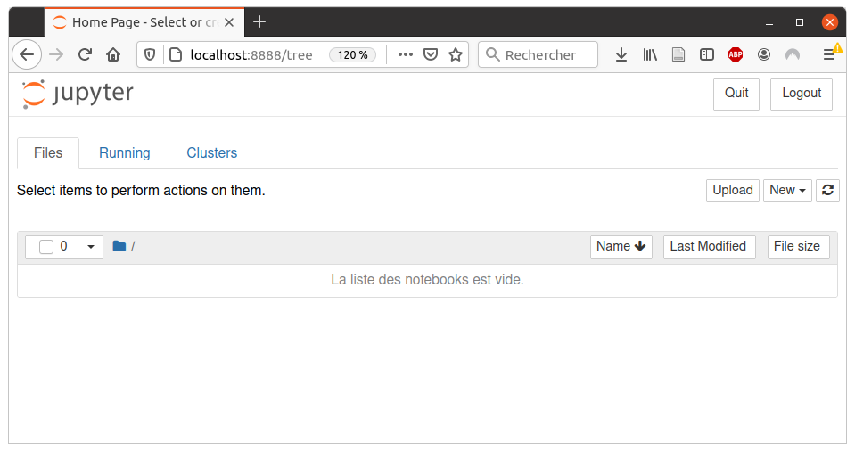
Si vous n'avez pas SageMath, vous pouvez suivre ces instructions du site jupyter.org. Ensuite, la commande jupyter notebook dans le terminal (Linux, OS X) ou dans l'invité de commande (Windows) vous permettra de l'ouvrir.
Vous devriez obtenir quelque chose qui ressemble à ceci dans votre navigateur:
JupyterLab:
Si vous avez déjà installé SageMath, vous pouvez installer JupyterLab en faisant sage -i jupyterlab et l'ouvrir en faisant sage -n jupyterlab. Sur Windows, c'est un tout petit peut différent, il faut plutôt faire pip install jupyterlab dans la console SageMath selon cette récente réponse sur ask.sagemath.org.
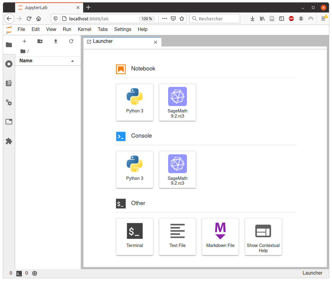
Si vous n'avez pas SageMath, vous pouvez suivre les instructions du même site que ci-haut. Ensuite, la commande jupyter-lab ou jupyter lab dans le terminal (Linux, OS X) ou dans l'invité de commande (Windows) vous permettra de l'ouvrir.
Vous devriez obtenir quelque chose qui ressemble à ceci dans votre navigateur:
Tiling a polyomino with polyominoes in SageMath
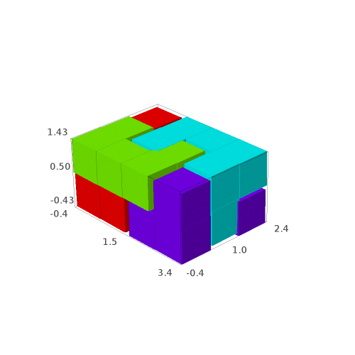
03 décembre 2020 | Catégories: sage, math | View CommentsSuppose that you 3D print many copies of the following 3D hexo-mino at home:
sage: from sage.combinat.tiling import Polyomino, TilingSolver
sage: p = Polyomino([(0,0,0), (0,1,0), (1,0,0), (2,0,0), (2,1,0), (2,1,1)], color='blue')
sage: p.show3d()
Launched html viewer for Graphics3d Object
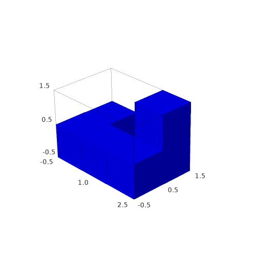
You would like to know if you can tile a larger polyomino or in particular a rectangular box with many copies of it. The TilingSolver module in SageMath is made for that. See also this recent question on ask.sagemath.org.
sage: T = TilingSolver([p], (7,5,3), rotation=True, reflection=False, reusable=True)
sage: T
Tiling solver of 1 pieces into a box of size 24
Rotation allowed: True
Reflection allowed: False
Reusing pieces allowed: True
There is no solution when tiling a box of shape 7x5x3 with this polyomino:
sage: T.number_of_solutions()
0
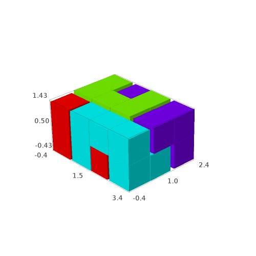
But there are 4 solutions when tiling a box of shape 4x3x2 with this polyomino:
sage: T = TilingSolver([p], (4,3,2), rotation=True, reflection=False, reusable=True)
sage: T.number_of_solutions()
4
We construct the list of solutions:
sage: solutions = [sol for sol in T.solve()]
Each solution contains the isometric copies of the polyominoes tiling the box:
sage: solutions[0]
[Polyomino: [(0, 0, 0), (0, 0, 1), (0, 1, 0), (1, 1, 0), (2, 0, 0), (2, 1, 0)], Color: #ff0000,
 Polyomino: [(0, 1, 1), (0, 2, 0), (0, 2, 1), (1, 1, 1), (2, 1, 1), (2, 2, 1)], Color: #ff0000,
 Polyomino: [(1, 0, 0), (1, 0, 1), (2, 0, 1), (3, 0, 0), (3, 0, 1), (3, 1, 0)], Color: #ff0000,
 Polyomino: [(1, 2, 0), (1, 2, 1), (2, 2, 0), (3, 1, 1), (3, 2, 0), (3, 2, 1)], Color: #ff0000]
It may be easier to visualize the solutions, so we define the following function allowing to draw the solutions with different colors for each piece:
sage: def draw_solution(solution, size=0.9):
....:     colors = rainbow(len(solution))
....:     for piece,col in zip(solution, colors):
....:         piece.color(col)
....:     return sum((piece.show3d(size=size) for piece in solution), Graphics())
sage: G = [draw_solution(sol) for sol in solutions]
sage: G
[Graphics3d Object, Graphics3d Object, Graphics3d Object, Graphics3d Object]
sage: G[0] # in Sage, this will open a 3d viewer automatically
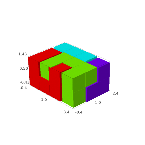
sage: G[1]
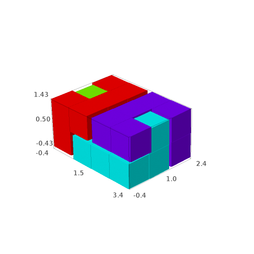
sage: G[2]
sage: G[3]
We may save the solutions to a file:
sage: G[0].save('solution0.png', aspect_ratio=1, zoom=1.2)
sage: G[1].save('solution1.png', aspect_ratio=1, zoom=1.2)
sage: G[2].save('solution2.png', aspect_ratio=1, zoom=1.2)
sage: G[3].save('solution3.png', aspect_ratio=1, zoom=1.2)
Question: are all of the 4 solutions isometric to each other?
The tiling problem is solved due to a reduction to the exact cover problem for which dancing links Knuth's algorithm provides all the solutions. One can see the rows of the dancing links matrix as follows:
sage: d = T.dlx_solver()
sage: d
Dancing links solver for 24 columns and 56 rows
sage: d.rows()
[[0, 1, 2, 4, 5, 11],
 [6, 7, 8, 10, 11, 17],
 [12, 13, 14, 16, 17, 23],
 ...
 [4, 6, 7, 9, 10, 11],
 [10, 12, 13, 15, 16, 17],
 [16, 18, 19, 21, 22, 23]]
The solutions to the dlx solver can be obtained as follows:
sage: it = d.solutions_iterator()
sage: next(it)
[3, 36, 19, 52]
These are the indices of the rows each corresponding to an isometric copy of the polyomino within the box.
Since SageMath-9.2, the possibility to reduce the problem to a MILP problem or a SAT instance was added to SageMath (see #29338 and #29955):
sage: d.to_milp()
(Boolean Program (no objective, 56 variables, 24 constraints),
 MIPVariable of dimension 1)
sage: d.to_sat_solver()
CryptoMiniSat solver: 56 variables, 2348 clauses.
Computer experiments for the Lyapunov exponent for MCF algorithms when dimension is larger than 3
27 mars 2020 | Catégories: sage, slabbe spkg, math | View CommentsIn November 2015, I wanted to share intuitions I developped on the behavior of various distinct Multidimensional Continued Fractions algorithms obtained from various kind of experiments performed with them often involving combinatorics and digitial geometry but also including the computation of their first two Lyapunov exponents.
As continued fractions are deeply related to the combinatorics of Sturmian sequences which can be seen as the digitalization of a straight line in the grid \(\mathbb{Z}^2\), the multidimensional continued fractions algorithm are related to the digitalization of a straight line and hyperplanes in \(\mathbb{Z}^d\).
This is why I shared those experiments in what I called 3-dimensional Continued Fraction Algorithms Cheat Sheets because of its format inspired from typical cheat sheets found on the web. All of the experiments can be reproduced using the optional SageMath package slabbe where I share my research code. People asked me whether I was going to try to publish those Cheat Sheets, but I was afraid the format would change the organization of the information and data in each page, so, in the end, I never submitted those Cheat Sheets anywhere.
Here I should say that \(d\) stands for the dimension of the vector space on which the involved matrices act and \(d-1\) is the dimension of the projective space on which the algorithm acts.
One of the consequence of the Cheat Sheets is that it made us realize that the algorithm proposed by Julien Cassaigne had the same first two Lyapunov exponents as the Selmer algorithm (first 3 significant digits were the same). Julien then discovered the explanation as its algorithm is conjugated to some semi-sorted version of the Selmer algorihm. This result was shared during WORDS 2017 conference. Julien Leroy, Julien Cassaigne and I are still working on the extended version of the paper. It is taking longer mainly because of my fault because I have been working hard on aperiodic Wang tilings in the previous 2 years.
During July 2019, Wolfgang, Valérie and Jörg asked me to perform computations of the first two Lyapunov exponents for \(d\)-dimensional Multidimensional Continued Fraction algorithms for \(d\) larger than 3. The main question of interest is whether the second Lyapunov exponent keeps being negative as the dimension increases. This property is related to the notion of strong convergence almost everywhere of the simultaneous diopantine approximations provided by the algorithm of a fixed vector of real numbers. It did not take me too long to update my package since I had started to generalize my code to larger dimensions during Fall 2017. It turns out that, as the dimension increases, all known MCF algorithms have their second Lyapunov exponent become positive. My computations were thus confirming what they eventually published in their preprint in November 2019.
My motivation for sharing the results is the conference Multidimensional Continued Fractions and Euclidean Dynamics held this week (supposed to be held in Lorentz Center, March 23-27 2020, it got cancelled because of the corona virus) where some discussions during video meetings are related to this subject.
The computations performed below can be summarized in one graphics showing the values of \(1-\theta_2/\theta_1\) with respect to \(d\) for various \(d\)-dimensional MCF algorithms. It seems that \(\theta_2\) is negative up to dimension 10 for Brun, up to dimension 4 for Selmer and up to dimension 5 for ARP.
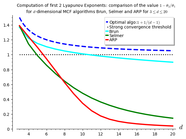
I have to say that I was disapointed by the results because the algorithm Arnoux-Rauzy-Poincaré (ARP) that Valérie and I introduced was not performing so well as its second Lyapunov exponent seems to become positive for dimension \(d\geq 6\). I had good expectations for ARP because it reaches the highest value for \(1-\theta_2/\theta_1\) in the computations performed in the Cheat Sheets, thus better than Brun, better than Selmer when \(d=3\).
The algorithm for the computation of the first two Lyapunov exponents was provided to me by Vincent Delecroix. It applies the algorithm \((v,w)\mapsto(M^{-1}v,M^T w)\) millions of times. The evolution of the size of the vector \(v\) gives the first Lyapunov exponent. The evolution of the size of the vector \(w\) gives the second Lyapunov exponent. Since the computation is performed on 64-bits double floating point number, their are numerical issues to deal with. This is why some Gramm Shimdts operation is performed on the vector \(w\) at each time the vectors are renormalized to keep the vector \(w\) orthogonal to \(v\). Otherwise, the numerical errors cumulate and the computed value for the \(\theta_2\) becomes the same as \(\theta_1\). You can look at the algorithm online starting at line 1723 of the file mult_cont_frac_pyx.pyx from my optional package.
I do not know from where Vincent took that algorithm. So, I do not know how exact it is and whether there exits any proof of lower bounds and upper bounds on the computations being performed. What I can say is that it is quite reliable in the sense that is returns the same values over and over again (by that I mean 3 common most significant digits) with any fixed inputs (number of iterations).
Below, I show the code illustrating how to reproduce the results.
The version 0.6 (November 2019) of my package slabbe includes the necessary code to deal with some \(d\)-dimensional Multidimensional Continued Fraction (MCF) algorithms. Its documentation is available online. It is a PIP package, so it can be installed like this:
sage -pip install slabbe
Recall that the dimension \(d\) below is the linear one and \(d-1\) is the dimension of the space for the corresponding projective algorithm.
Import the Brun, Selmer and Arnoux-Rauzy-Poincaré MCF algorithms from the optional package:
sage: from slabbe.mult_cont_frac import Brun, Selmer, ARP
The computation of the first two Lyapunov exponents performed on one single orbit:
sage: Brun(dim=3).lyapunov_exponents(n_iterations=10^7)
(0.30473782969922547, -0.11220958022368056, 1.3682167728713919)
The starting point is taken randomly, but the results of the form of a 3-tuple \((\theta_1,\theta_2,1-\theta_2/\theta_1)\) are about the same:
sage: Brun(dim=3).lyapunov_exponents(n_iterations=10^7)
(0.30345018206132324, -0.11171509867725296, 1.3681497170915415)
Increasing the dimension \(d\) yields:
sage: Brun(dim=4).lyapunov_exponents(n_iterations=10^7)
(0.32639514522732005, -0.07191456560115839, 1.2203297648654456)
sage: Brun(dim=5).lyapunov_exponents(n_iterations=10^7)
(0.30918877340506756, -0.0463930802132972, 1.1500477514185734)
It performs an orbit of length \(10^7\) in about .5 seconds, of length \(10^8\) in about 5 seconds and of length \(10^9\) in about 50 seconds:
sage: %time Brun(dim=3).lyapunov_exponents(n_iterations=10^7)
CPU times: user 540 ms, sys: 0 ns, total: 540 ms
Wall time: 539 ms
(0.30488799356325225, -0.11234354880132114, 1.3684748208296182)
sage: %time Brun(dim=3).lyapunov_exponents(n_iterations=10^8)
CPU times: user 5.09 s, sys: 0 ns, total: 5.09 s
Wall time: 5.08 s
(0.30455473631148755, -0.11217550411862384, 1.3683262505689446)
sage: %time Brun(dim=3).lyapunov_exponents(n_iterations=10^9)
CPU times: user 51.2 s, sys: 0 ns, total: 51.2 s
Wall time: 51.2 s
(0.30438755982577026, -0.11211562816821799, 1.368331834035505)
Here, in what follows, I must admit that I needed to do a small fix to my package, so the code below will not work in version 0.6 of my package, I will update my package in the next days in order that the computations below can be reproduced:
sage: from slabbe.lyapunov import lyapunov_comparison_table
For each \(3\leq d\leq 20\), I compute 30 orbits and I show the most significant digits and the standard deviation of the 30 values computed.
For Brun algorithm:
sage: algos = [Brun(d) for d in range(3,21)]
sage: %time lyapunov_comparison_table(algos, n_orbits=30, n_iterations=10^7, ncpus=8)
CPU times: user 190 ms, sys: 2.8 s, total: 2.99 s
Wall time: 6min 31s
  Algorithm     \#Orbits   $\theta_1$ (std)     $\theta_2$ (std)      $1-\theta_2/\theta_1$ (std)
+-------------+----------+--------------------+---------------------+-----------------------------+
  Brun (d=3)    30         0.3045 (0.00040)     -0.1122 (0.00017)     1.3683 (0.00022)
  Brun (d=4)    30         0.32632 (0.000055)   -0.07188 (0.000051)   1.2203 (0.00014)
  Brun (d=5)    30         0.30919 (0.000032)   -0.04647 (0.000041)   1.1503 (0.00013)
  Brun (d=6)    30         0.28626 (0.000027)   -0.03043 (0.000035)   1.1063 (0.00012)
  Brun (d=7)    30         0.26441 (0.000024)   -0.01966 (0.000027)   1.0743 (0.00010)
  Brun (d=8)    30         0.24504 (0.000027)   -0.01207 (0.000024)   1.04926 (0.000096)
  Brun (d=9)    30         0.22824 (0.000021)   -0.00649 (0.000026)   1.0284 (0.00012)
  Brun (d=10)   30         0.2138 (0.00098)     -0.0022 (0.00015)     1.0104 (0.00074)
  Brun (d=11)   30         0.20085 (0.000015)   0.00106 (0.000022)    0.9947 (0.00011)
  Brun (d=12)   30         0.18962 (0.000017)   0.00368 (0.000021)    0.9806 (0.00011)
  Brun (d=13)   30         0.17967 (0.000011)   0.00580 (0.000020)    0.9677 (0.00011)
  Brun (d=14)   30         0.17077 (0.000011)   0.00755 (0.000021)    0.9558 (0.00012)
  Brun (d=15)   30         0.16278 (0.000012)   0.00900 (0.000017)    0.9447 (0.00010)
  Brun (d=16)   30         0.15556 (0.000011)   0.01022 (0.000013)    0.93433 (0.000086)
  Brun (d=17)   30         0.149002 (9.5e-6)    0.01124 (0.000015)    0.9246 (0.00010)
  Brun (d=18)   30         0.14303 (0.000010)   0.01211 (0.000019)    0.9153 (0.00014)
  Brun (d=19)   30         0.13755 (0.000012)   0.01285 (0.000018)    0.9065 (0.00013)
  Brun (d=20)   30         0.13251 (0.000011)   0.01349 (0.000019)    0.8982 (0.00014)
For Selmer algorithm:
sage: algos = [Selmer(d) for d in range(3,21)]
sage: %time lyapunov_comparison_table(algos, n_orbits=30, n_iterations=10^7, ncpus=8)
CPU times: user 203 ms, sys: 2.78 s, total: 2.98 s
Wall time: 6min 27s
  Algorithm       \#Orbits   $\theta_1$ (std)     $\theta_2$ (std)      $1-\theta_2/\theta_1$ (std)
+---------------+----------+--------------------+---------------------+-----------------------------+
  Selmer (d=3)    30         0.1827 (0.00041)     -0.0707 (0.00017)     1.3871 (0.00029)
  Selmer (d=4)    30         0.15808 (0.000058)   -0.02282 (0.000036)   1.1444 (0.00023)
  Selmer (d=5)    30         0.13199 (0.000033)   0.00176 (0.000034)    0.9866 (0.00026)
  Selmer (d=6)    30         0.11205 (0.000017)   0.01595 (0.000036)    0.8577 (0.00031)
  Selmer (d=7)    30         0.09697 (0.000012)   0.02481 (0.000030)    0.7442 (0.00032)
  Selmer (d=8)    30         0.085340 (8.5e-6)    0.03041 (0.000032)    0.6437 (0.00036)
  Selmer (d=9)    30         0.076136 (5.9e-6)    0.03379 (0.000032)    0.5561 (0.00041)
  Selmer (d=10)   30         0.068690 (5.5e-6)    0.03565 (0.000023)    0.4810 (0.00032)
  Selmer (d=11)   30         0.062557 (4.4e-6)    0.03646 (0.000021)    0.4172 (0.00031)
  Selmer (d=12)   30         0.057417 (3.6e-6)    0.03654 (0.000017)    0.3636 (0.00028)
  Selmer (d=13)   30         0.05305 (0.000011)   0.03615 (0.000018)    0.3186 (0.00032)
  Selmer (d=14)   30         0.04928 (0.000060)   0.03546 (0.000051)    0.2804 (0.00040)
  Selmer (d=15)   30         0.046040 (2.0e-6)    0.03462 (0.000013)    0.2482 (0.00027)
  Selmer (d=16)   30         0.04318 (0.000011)   0.03365 (0.000014)    0.2208 (0.00028)
  Selmer (d=17)   30         0.040658 (3.3e-6)    0.03263 (0.000013)    0.1974 (0.00030)
  Selmer (d=18)   30         0.038411 (2.7e-6)    0.031596 (9.8e-6)     0.1774 (0.00022)
  Selmer (d=19)   30         0.036399 (2.2e-6)    0.030571 (8.0e-6)     0.1601 (0.00019)
  Selmer (d=20)   30         0.0346 (0.00011)     0.02955 (0.000093)    0.1452 (0.00019)
For Arnoux-Rauzy-Poincaré algorithm:
sage: algos = [ARP(d) for d in range(3,21)]
sage: %time lyapunov_comparison_table(algos, n_orbits=30, n_iterations=10^7, ncpus=8)
CPU times: user 226 ms, sys: 2.76 s, total: 2.99 s
Wall time: 13min 20s
  Algorithm                        \#Orbits   $\theta_1$ (std)     $\theta_2$ (std)      $1-\theta_2/\theta_1$ (std)
+--------------------------------+----------+--------------------+---------------------+-----------------------------+
  Arnoux-Rauzy-Poincar\'e (d=3)    30         0.4428 (0.00056)     -0.1722 (0.00025)     1.3888 (0.00016)
  Arnoux-Rauzy-Poincar\'e (d=4)    30         0.6811 (0.00020)     -0.16480 (0.000085)   1.24198 (0.000093)
  Arnoux-Rauzy-Poincar\'e (d=5)    30         0.7982 (0.00012)     -0.0776 (0.00010)     1.0972 (0.00013)
  Arnoux-Rauzy-Poincar\'e (d=6)    30         0.83563 (0.000091)   0.0475 (0.00010)      0.9432 (0.00012)
  Arnoux-Rauzy-Poincar\'e (d=7)    30         0.8363 (0.00011)     0.1802 (0.00016)      0.7845 (0.00020)
  Arnoux-Rauzy-Poincar\'e (d=8)    30         0.8213 (0.00013)     0.3074 (0.00023)      0.6257 (0.00028)
  Arnoux-Rauzy-Poincar\'e (d=9)    30         0.8030 (0.00012)     0.4205 (0.00017)      0.4763 (0.00022)
  Arnoux-Rauzy-Poincar\'e (d=10)   30         0.7899 (0.00011)     0.5160 (0.00016)      0.3467 (0.00020)
  Arnoux-Rauzy-Poincar\'e (d=11)   30         0.7856 (0.00014)     0.5924 (0.00020)      0.2459 (0.00022)
  Arnoux-Rauzy-Poincar\'e (d=12)   30         0.7883 (0.00010)     0.6497 (0.00012)      0.1759 (0.00014)
  Arnoux-Rauzy-Poincar\'e (d=13)   30         0.7930 (0.00010)     0.6892 (0.00014)      0.1309 (0.00014)
  Arnoux-Rauzy-Poincar\'e (d=14)   30         0.7962 (0.00012)     0.7147 (0.00015)      0.10239 (0.000077)
  Arnoux-Rauzy-Poincar\'e (d=15)   30         0.7974 (0.00012)     0.7309 (0.00014)      0.08340 (0.000074)
  Arnoux-Rauzy-Poincar\'e (d=16)   30         0.7969 (0.00015)     0.7411 (0.00014)      0.07010 (0.000048)
  Arnoux-Rauzy-Poincar\'e (d=17)   30         0.7960 (0.00014)     0.7482 (0.00014)      0.06005 (0.000050)
  Arnoux-Rauzy-Poincar\'e (d=18)   30         0.7952 (0.00013)     0.7537 (0.00014)      0.05218 (0.000046)
  Arnoux-Rauzy-Poincar\'e (d=19)   30         0.7949 (0.00012)     0.7584 (0.00013)      0.04582 (0.000035)
  Arnoux-Rauzy-Poincar\'e (d=20)   30         0.7948 (0.00014)     0.7626 (0.00013)      0.04058 (0.000025)
The computation of the figure shown above is done with the code below:
sage: brun_list = [1.3683, 1.2203, 1.1503, 1.1063, 1.0743, 1.04926, 1.0284, 1.0104, 0.9947, 0.9806, 0.9677, 0.9558, 0.9447, 0.93433, 0.9246, 0.9153, 0.9065, 0.8982]
sage: selmer_list = [ 1.3871, 1.1444, 0.9866, 0.8577, 0.7442, 0.6437, 0.5561, 0.4810, 0.4172, 0.3636, 0.3186, 0.2804, 0.2482, 0.2208, 0.1974, 0.1774, 0.1601, 0.1452]
sage: arp_list = [1.3888, 1.24198, 1.0972, 0.9432, 0.7845, 0.6257, 0.4763, 0.3467, 0.2459, 0.1759, 0.1309, 0.10239, 0.08340, 0.07010, 0.06005, 0.05218, 0.04582, 0.04058]
sage: brun_points = list(enumerate(brun_list, start=3))
sage: selmer_points = list(enumerate(selmer_list, start=3))
sage: arp_points = list(enumerate(arp_list, start=3))
sage: G = Graphics()
sage: G += plot(1+1/(x-1), x, 3, 20, legend_label='Optimal algo:$1+1/(d-1)$', linestyle='dashed', color='blue', thickness=3)
sage: G += line([(3,1), (20,1)], color='black', legend_label='Strong convergence threshold', linestyle='dotted', thickness=2)
sage: G += line(brun_points, legend_label='Brun', color='cyan', thickness=3)
sage: G += line(selmer_points, legend_label='Selmer', color='green', thickness=3)
sage: G += line(arp_points, legend_label='ARP', color='red', thickness=3)
sage: G.ymin(0)
sage: G.axes_labels(['$d$',''])
sage: G.show(title='Computation of first 2 Lyapunov Exponents: comparison of the value $1-\\theta_2/\\theta_1$\n for $d$-dimensional MCF algorithms Brun, Selmer and ARP for $3\\leq d\\leq 20$')
« Previous Page -- Next Page »
Propulsé par Blogofile
S'abonner au Flux RSS
et aux Commentaires.

This work by Sébastien Labbé is licensed under a Creative Commons Attribution-ShareAlike 4.0 International License.