Percolation and self-avoiding walks
18 décembre 2012 | Mise à jour: 20 décembre 2012 | Catégories: sage | View CommentsToday, I am presenting the Chapter 3 of the book Probability on Graphs of Geoffrey Grimmett during a monthly reading seminar at LIAFA. The title of the chapter is Percolation and self-avoiding walks. I did some computations to improve my intuition on the question. My code is in the following file : bond_percolation.sage. This post is about some of my computations. You might want to test them yourself online using the Sage Cell Server.
Basic Definitions
Let \(\mathbb{L}^d=(\mathbb{Z}^d,\mathbb{E}^d)\) be the hypercubic lattice. Let \(p\in[0,1]\). Each edge \(e\in \mathbb{E}^d\) is designated either open with probability \(p\), or closed otherwise, different edges receiving independant states. For \(x,y\in \mathbb{Z}^d\), we write \(x \leftrightarrow y \) if there exists an open path joining \(x\) and \(y\). For \(x\in \mathbb{Z}^d\), we consider the open cluster \(C_x\) containing \(x\) : \[ C_x = \{y \in \mathbb{Z}^d : x \leftrightarrow y \}. \] The percolation probability \(\Theta(p)\) is given by \[ \Theta(p) = P_p(\vert C_0\vert=\infty). \] Finally, the critical probability is defined as \[ p_c = \sup\{p : \Theta(p) = 0 \}. \] The question is to compute \(p_c\). Results in the Chapter give lower bound and upper bound for \(p_c\). Many problems are still open like the one claiming that \(\Theta(p_c) = 0\) for all \(d\geq 2\): it is known only for \(d=2\) and \(d\geq 19\) according to a remark in the chapter.
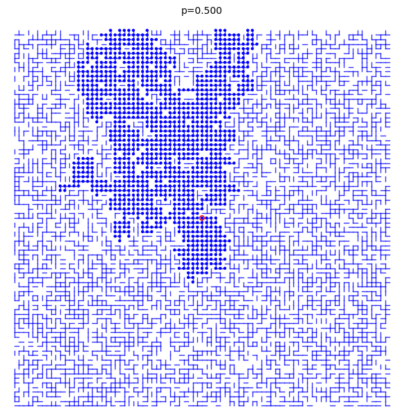
Some samples when p=0.5
A bond percolation sample inside the box \(\Lambda(m)=[-m,m]^d\) when \(p=0.5\) and \(d=2\):
sage: S = BondPercolationSample(p=0.5, d=2)
sage: S.plot(m=40, pointsize=10, thickness=1)
Graphics object consisting of 7993 graphics primitives
sage: _.show()
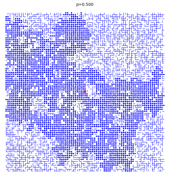
Another time gives something different:
sage: S = BondPercolationSample(p=0.5, d=2)
sage: S.plot(m=40, pointsize=10, thickness=1)
Graphics object consisting of 10176 graphics primitives
sage: _.show()
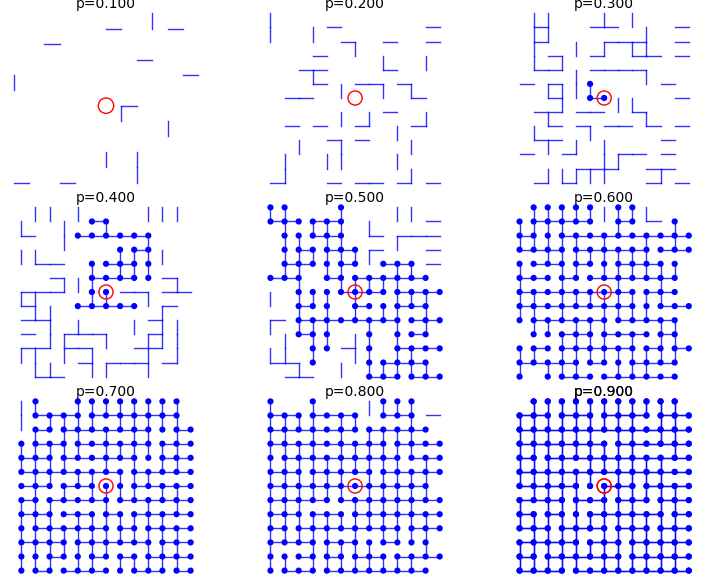
Some samples for ranges of values of p
From p=0.1 to p=0.9:
sage: percolation_graphics_array(srange(0.1,1,0.1), d=2, m=5)
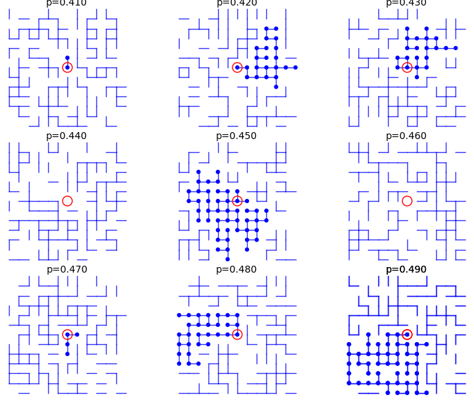
From p=0.41 to p=0.49:
sage: percolation_graphics_array(srange(0.41,0.50,0.01), d=2, m=5)
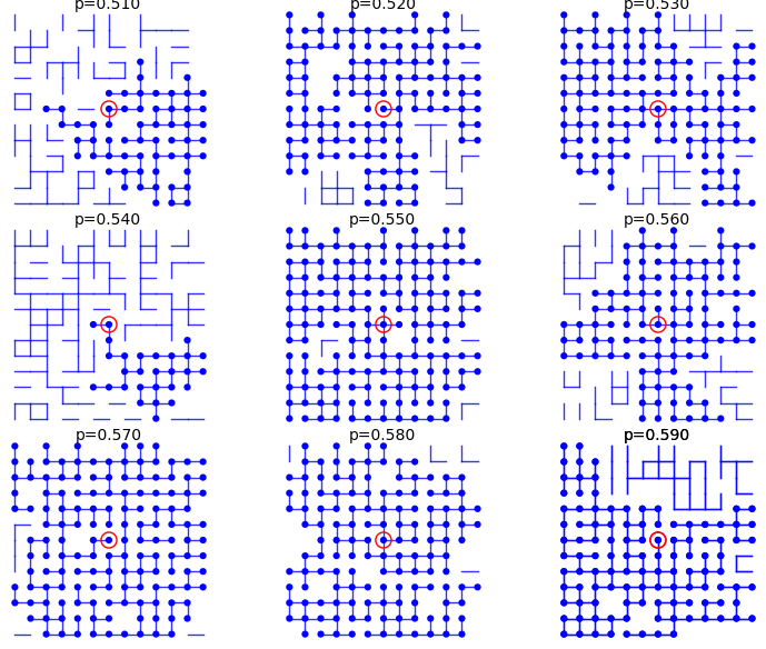
From p=0.51 to p=0.59:
sage: percolation_graphics_array(srange(0.51,0.60,0.01), d=2, m=5)
Upper bound and lower bound for percolation probability \(\Theta(p)\)
In every case, we have the following upper bound for the percolation probability: \[ \Theta(p) = \mathbb{P}_p(\vert C_0\vert=\infty) \leq \mathbb{P}_p(\vert C_0\vert > 1) = 1 - \mathbb{P}_p(\vert C_0\vert = 1) = 1 - (1-p)^{2d}. \] In particular, if \(p\neq 1\), then \(\Theta(p)<1\). In Sage, define the upper bound:
sage: p,n = var('p,n')
sage: d = var('d')
sage: upper_bound = 1 - (1-p)^(2*d)
Also, from Equation (3.8), we have the following lower bound: \[ \Theta(p) \geq 1 - \sum_{n=4}^{\infty} n (4(1-p))^n. \]
In Sage, define the lower bound:
sage: p,n = var('p,n')
sage: lower_bound = 1 - sum(n*(4*(1-p))^n,n,4,oo)
sage: lower_bound.factor()
-(3072*p^5 - 14336*p^4 + 26624*p^3 - 24592*p^2 + 11288*p - 2057)/(4*p - 3)^2
This is not defined when \(p=3/4\), but we are interested in the values in the interval \(]3/4,1]\). In particular, for which value of \(p\) is this lower bound strictly larger than zero:
sage: root = lower_bound.find_root(0.76, 0.99); root
0.8639366490304586
Let's now draw a graph of the lower and upper bound:
sage: U = plot(upper_bound(d=2),(0,1),color='red', thickness=3)
sage: L = plot(lower_bound,(0.86,1),color='green', thickness=3)
sage: G = U + L
sage: G += point((root, 0), color='red', size=20)
sage: lower = r"$1-\sum_{n=4}^{\infty} n4^n(1-p)^n$"
sage: upper = r"$1 -(1-p)^{4}$"
sage: title = r"$1-\sum_{n=4}^{\infty} n4^n(1-p)^n\leq\Theta(p)\leq 1 -(1-p)^{2d}$"
sage: G += text(title, (.5, 1.05), color='black', fontsize=15)
sage: G += text(upper, (.3, 0.5), color='red', fontsize=20)
sage: G += text(lower, (.7, 0.5), color='green', fontsize=20)
sage: G += text("%.5f"%root,(0.88, .03), color='green', horizontal_alignment='left')
sage: G.show()
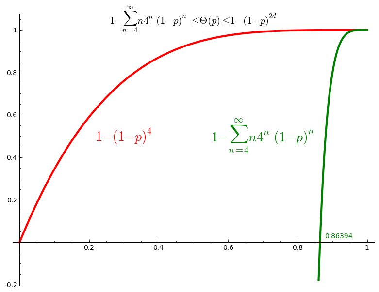
Thus we conclude that \(\Theta(p) >0\) for \(p>0.8639\) and thus \(p_c \leq 0.8639\).
Percolation probability - dimension 2
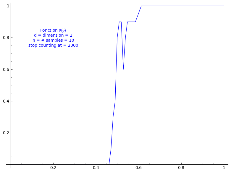
The code allows to define the percolation probability function for a given dimension d. It generates n samples and consider the cluster to be infinite if its cardinality is larger than the given stop value.
Here we use Sage adaptative recursion algorithm for drawing the plot of the percolation probability which finds the particular important intervals to ask for more values of the function. See help section of plot function for details. Because T might be long to compute we start with only 4 points.
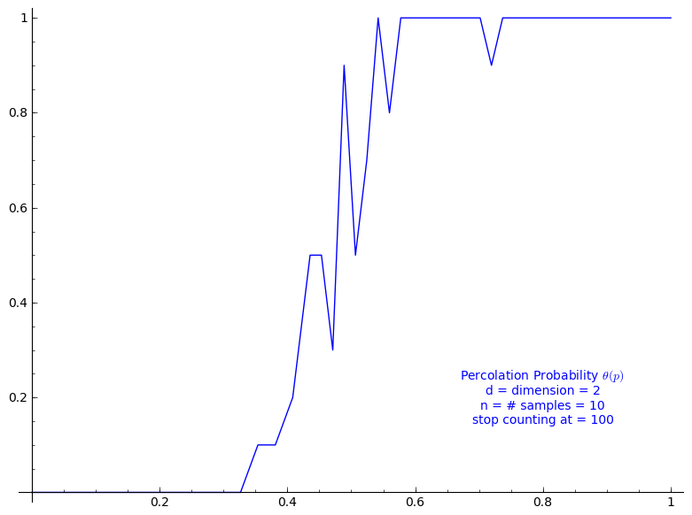
When stop=100:
sage: T = PercolationProbability(d=2, n=10, stop=100)
sage: T.return_plot((0,1),adaptive_recursion=4,plot_points=4).show()
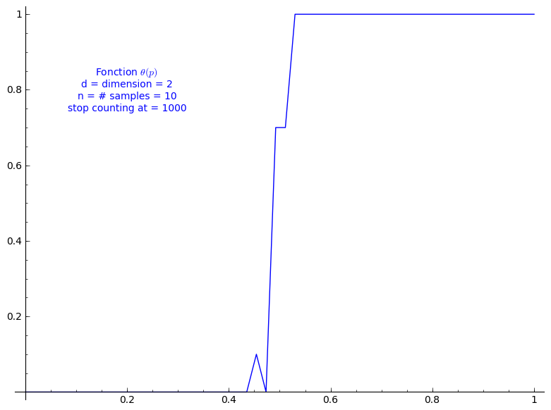
When stop=1000:
sage: T = PercolationProbability(d=2, n=10, stop=1000)
sage: T.return_plot((0,1),adaptive_recursion=4,plot_points=4).show()
When stop=2000:
sage: T = PercolationProbability(d=2, n=10, stop=2000)
sage: T.return_plot((0,1),adaptive_recursion=4,plot_points=4).show()
Percolation probability - dimension 3
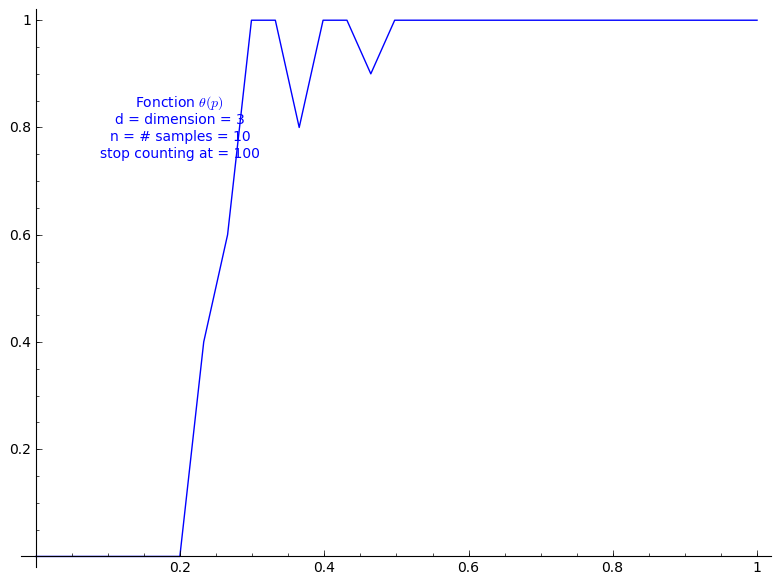
When stop=100:
sage: T = PercolationProbability(d=3, n=10, stop=100)
sage: T.return_plot((0,1),adaptive_recursion=4,plot_points=4).show()
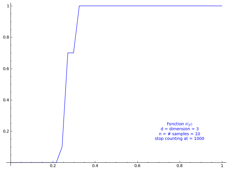
When stop=1000:
sage: T = PercolationProbability(d=3, n=10, stop=1000)
sage: T.return_plot((0,1),adaptive_recursion=4,plot_points=4).show()
Percolation probability - dimension 4
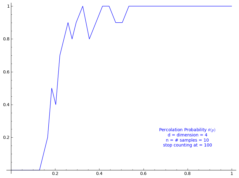
When stop=100:
sage: T = PercolationProbability(d=4, n=10, stop=100)
sage: T.return_plot((0,1),adaptive_recursion=4,plot_points=4).show()
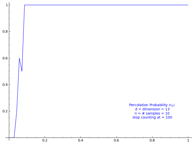
Percolation probability - dimension 13
When stop=100:
sage: T = PercolationProbability(d=13, n=10, stop=100)
sage: T.return_plot((0,1),adaptive_recursion=4,plot_points=4).show()
Theorem 3.2
Theorem 3.2 states that \(0 < p_c < 1\), but its proof does much more in fact. Following the computation we just did for Equation (3.8), we get for \(d=2\) \[ 0.3333 < \frac{1}{2d-1} \leq p_c \leq 0.8639 \] and for \(d=3\): \[ 0.2000 < \frac{1}{2d-1} \leq p_c \leq 0.8639 \] This allows to grasp the improvement brought later by Theorem 3.12.
Connective constant
Using the two following sequences of the On-Line Encyclopedia of Integer Sequences, one can evaluate the connective constant \(\kappa(d)\)
By taking the k-th root of of k-th term of A001411, we may give an approximation of \(\kappa(2)\):
sage: L = [1, 4, 12, 36, 100, 284, 780, 2172, 5916, 16268, 44100, 120292,
324932, 881500, 2374444, 6416596, 17245332, 46466676, 124658732, 335116620,
897697164, 2408806028, 6444560484, 17266613812, 46146397316, 123481354908,
329712786220, 881317491628]
sage: for k in range(1, len(L)): print numerical_approx(L[k]^(1/k))
4.00000000000000
3.46410161513775
3.30192724889463
3.16227766016838
3.09502148400370
3.03400133198980
2.99705187539871
2.96144397263395
2.93714926770637
2.91369345857619
2.89627439045790
2.87949308754677
2.86632078916860
2.85362749495679
2.84328447096562
2.83329615650289
2.82493415671599
2.81684125361654
2.80992368218258
2.80321554383456
2.79738645741910
2.79172363211806
2.78673687369245
2.78188437392354
2.77756387722633
2.77335345579129
2.76956977331575
By taking the k-th root of of k-th term of A001412, we may give an approximation of \(\kappa(3)\):
sage: L = [1, 6, 30, 150, 726, 3534, 16926, 81390, 387966, 1853886,
8809878, 41934150, 198842742, 943974510, 4468911678, 21175146054,
100121875974, 473730252102, 2237723684094, 10576033219614, 49917327838734,
235710090502158, 1111781983442406, 5245988215191414, 24730180885580790,
116618841700433358, 549493796867100942,2589874864863200574,
12198184788179866902, 57466913094951837030, 270569905525454674614]
sage: for k in range(1, len(L)): print numerical_approx(L[k]^(1/k))
6.00000000000000
5.47722557505166
5.31329284591305
5.19079831727404
5.12452137580198
5.06709510955294
5.02933019629493
4.99573287588832
4.97111339009676
4.94876680377358
4.93129192790635
4.91521453865211
4.90209314463520
4.88990167518413
4.87964724632057
4.87004597517131
4.86178722582108
4.85400655861169
4.84719703702142
4.84074902256992
4.83502763526502
4.82958688248615
4.82470487210973
4.82004549244633
4.81582557693112
4.81178552451599
4.80809774735294
4.80455755518719
4.80130435575213
4.79817388859565
Then, \(\kappa(2)\) would be something less than 2.769 and \(\kappa(3)\) would be something less than 4.798.
Theorem 3.12
Thus, we may evaluate the lower bound and upper bound given at Theorem 3.12. For dimension \(d=2\):
sage: k < 2.76956977331575
k < 2.76956977331575
sage: _ / (2.76956977331575  * k)
0.361066909970928 < (1/k)
sage: 1 - 0.361066909970928
0.638933090029072
The critical probability of bond percolation on \(\mathbb{L}^d\) with \(d=2\) satisfies \[ 0.3610 < \frac{1}{\kappa(2)} \leq p_c \leq 1 - \frac{1}{\kappa(2)} < 0.6389. \] If we look at the graph of the percolation probability \(\Theta(p)\) we did above for when \(d=2\), it seems that the lower bound is not far from \(p_c\). The lower bound 0.3610 is a small improvement to the simple one got from Theorem 3.2 (0.3333).
Similarly, for dimension \(d=3\):
sage: k < 4.79817388859565
k < 4.79817388859565
sage: _ / (4.79817388859565 * k)
0.208412621805310 < (1/k)
The critical probability of bond percolation on \(\mathbb{L}^d\) with \(d=3\) satisfies \[ 0.2084 < \frac{1}{\kappa(3)} \leq p_c \leq 1 - \frac{1}{\kappa(2)} < 0.6389. \] Again, if we look at the graph of \(\Theta(p)\) we did above for when \(d=3\), it seems that the lower bound 0.2084 is not far from \(p_c\). In this case, the lower bound 0.2084 is a rather small improvement to the lower bound from Theorem 3.2 (0.2000). It might be caused by a poor approximation of \(\kappa(3)\) from the above sequences of only 30 terms from the OEIS.
Some small Sage tricks
14 décembre 2012 | Catégories: sage | View CommentsBelow are some Sage tricks that I gathered from other users of Sage, from sage-devel and other places since one year.
Stop the focus in the Notebook
This Notebook hack of the day was published on sage-devel by William Stein during May 2012 to fix that focus movement in the Notebook:
html('<script>cell_focus=function(x,y){} </script>')
Consult the documentation of a function in the browser
Open the documentation of a particular function in a web browser, from either the command-line or the notebook:
sage: browse_sage_doc(factor)
It works also for methods of an object:
sage: m = matrix(2, range(4))
sage: browse_sage_doc(m.inverse)
I found this command when I consulted the help():
sage: help()
Implicit multiplication
Some behavior in Sage can be made implicit like multiplication and variable definition. This might be good for new users coming from Maple for instance.
Normally, this syntax raises an error:
sage: 34x
------------------------------------------------------------
   File "<ipython console>", line 1
     34x
       ^
SyntaxError: invalid syntax
It is possible to make it work:
sage: implicit_multiplication(True)
sage: 34x
34*x
Implicit variable definition
The following works only in the Sage Notebook. It allows to turn on automatic definition of variables:
sage: automatic_names(True)
sage: x + y + z
x + y + z
Turn out automatic show when using plot
Set the default to False for showing plots using any plot commands:
sage: show_default(False)
I prefer False but you may not.
Rerun the patchbot
One can re-run the tests of a particular ticket by adding ?kick to the url of the ticket on the patchbot Sage server. For example, to rerun the tests on the ticket #13461, one can load the following page:
http://patchbot.sagemath.org/ticket/13461/?kick
This trick was shared on sage-devel during August 2012.
Python debugger
The majority of the Best Practices for Scientific Computing are followed by the Sage Development model. But, there is one principle that at least I do not use enough : a debugger. However, a Python debugger exists and a tutorial for using the Python debugger is available on onlamp.com.
I remember that discussion on sage-devel Poll: which debugger do you use? where developers were sharing their debugger tricks. It seems that using print statements is unavoidable.
Computing basic statistics with R
I always knew R is in Sage but never used it even if sometimes I need to compute some statistics of list of numbers. In Sage, one can print statistics of a list of numbers using R:
sage: L = [randint(0,100) for _ in range(20)]
sage: r.summary(L)
   Min. 1st Qu.  Median    Mean 3rd Qu.    Max.
  14.00   27.75   57.50   53.45   69.00   98.00
Creation of the number field in \(\sqrt{5}\)
Before learning it from this video of William Stein, I did not know that the square brackets could be used to create such number field:
sage: A = ZZ[sqrt(5)]
sage: a,sqrt5 = A.gens()
sage: A
Order in Number Field in sqrt5 with defining polynomial x^2 - 5
sage: sqrt5
sqrt5
Using Sage locally in the notebook from a server
First, log into the server using the following port setup:
ssh -L 8389:localhoat:8389 [SERVER]
Start the notebook with the given port:
sage -notebook port=8389
This ask for a password, if you forget it, you may reset it by first opening Sage, and by starting the notebook with the option reset=True:
sage: notebook(port=8389, reset=True)
Then, by opening the browser at the following adress, I can log in to the notebook from the server:
http://localhost:8389/home/admin/
Going from Mercurial to Git
Sage will soon move from Mercurial to Git. In the past, I tried to understand the difference between Mercurial and Git. I was never able to find a simple text or blog post on the web explaining in a simple way the differences. One diffence would be about branching. But I was not using branches with Mercurial... As I see it, differences between Mercurial and Git are hard to explain or at least hard to understand.
Anyway, I once found this tutorial on the Git version control system: Understanding Git Conceptually where the approach is "conceptual" and maybe easier for the mathematician. For instance, in Section 1 it is written that repositories can be "visualized as a directed acyclic graph of commit objects". I still haven't go through this tutorial but I consider to start with this one.
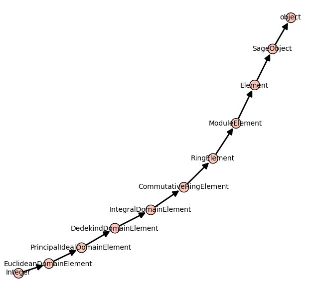
Inheritance tree
One may draw the inheritance tree of a class with the following command:
sage: class_graph(Integer).plot()
Blogofile, un générateur de site web statique
28 novembre 2012 | Catégories: web | View CommentsLa toute dernière version de Blogofile 0.8.b vient de sortir plus d'un an après la version 0.7.1 que j'utilise pour ce site web. Blogofile est un générateur de site web statique, c'est-à-dire qui dépend uniquement de fichiers textes. Il existe une multitude de projets similaires dont Pelican, nanoc, Octopress, Cytoplasm, rstblog et plusieurs autres. Le site web mathematism.com a fait le choix de nanoc et mickgardner.com a choisi Jekyll. Un autre a choisi de coder son propre ReStructuredText-Writer en le basant sur docutils.
Pour ma part, j'ai choisi Blogofile, car il est basé sur le langage Python, comprend la syntaxe ReStructuredText et aussi parce que j'ai été capable de l'utiliser dès la première journée contrairement au projet Hyde aussi basé sur Python, mais que je n'ai jamais réussi à comprendre.
D'autres personnes ont fait le même choix que moi tel que le créateur de Mako Templates qui explique son choix dans son texte how coders blog ainsi que ses blogofile hacks. Finalement, voici trois autres sites qui expliquent leur passage à blogofile: asktherelic.com, paolocorti.net et lukeplant.me.uk.
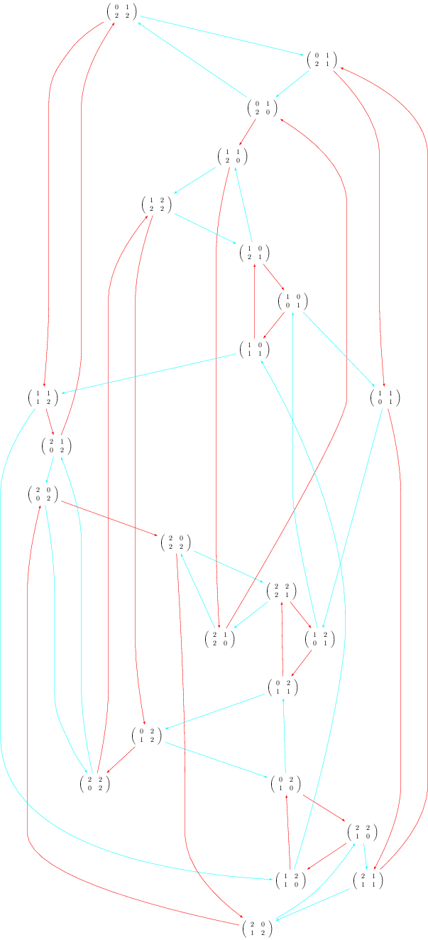
Using Sage + graphviz + dot2tex + tikz + tikz2pdf to draw a graph
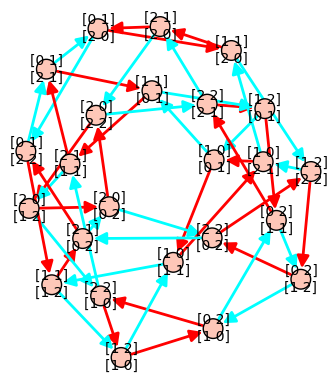
13 novembre 2012 | Mise à jour: 16 novembre 2012 | Catégories: latex, sage | View CommentsLet's first construct a graph that we will use in our examples below. We first construct a finite group generated by 2 by 2 matrices on the field \(GF(3)\). The group contains 24 elements. We then construct its Cayley graph:
sage: F = GF(3)
sage: gens = [matrix(F,2,[1,0, 1,1]), matrix(F,2, [1,1, 0,1])]
sage: group = MatrixGroup(gens); group
Matrix group over Finite Field of size 3 with 2 generators:
[[[1, 0], [1, 1]], [[1, 1], [0, 1]]]
sage: group.cardinality()
24
sage: G = group.cayley_graph()
Default graph plot
The default graph plot in Sage is:
sage: G.show(color_by_label=True)
Using view is actually broken when vertices are matrices because default format (format='tkz_graph') does not support it:
sage: view(G)
An error occurred.
...
LaTex error
Installing dot2tex + graphviz
One may get another kind of tikz output using the dot2tex.spkg together with graphviz. To know what is the latest available version of dot2tex use the command optional_packages():
sage: [x for x in flatten(optional_packages()) if 'dot2tex' in x]
['dot2tex-2.8.7-2']
The command to install the most recent version of dot2tex.spkg do from the command line (where you replace the version numbers by the above output):
sage -i dot2tex-2.8.7-2
As the documentation of G.layout_graphviz() says, install graphviz >= 2.14 so that the programs dot, neato, ... are in your path. The graphviz suite can be download from the graphviz website.
Basic Usage
This should allow the following to work:
sage: G.set_latex_options(format='dot2tex', prog='neato')
sage: G.set_latex_options(color_by_label=True)
sage: view(G)
Limits of the basic usage
With the above usage, you will find that the command view(G) command is very slow and that sometimes it just doesn't work and gives a Latex error like this:
sage: G.set_latex_options(format='dot2tex', prog='dot')
sage: view(G)
An error occurred.
...
LaTex error
This is because the default compilation is just unappropriate for our usage (I still wonder for which usage it can be appropriate). In fact, the default compilation is first trying the conversion tex to dvi to png using latex and dvipng. If the dvipng part does not work for whatever reason (which is our case), it will then try the conversion dvi to ps to pdf using dvips and ps2pdf. This worked above for prog='neato' but not for prog='dot' because dvipng does not seem to like when latex produces Overfull \hbox and Overfull \vbox.
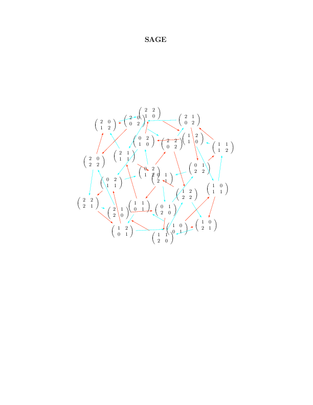
The Best Usage
The compilation strategy can be changed by using the engine option and by setting it to 'pdflatex'. Also the Overfull problem can be solved using the option tightpage=True:
sage: G.set_latex_options(format='dot2tex', prog='dot')
sage: G.set_latex_options(color_by_label=True)
sage: view(G, engine='pdflatex', tightpage=True)
More options
The variable prog is for the program used for the layout. It must be a string corresponding to one of the software of the graphviz suite. Accepted values for prog are:
- 'dot' (the default)
- 'neato'
- 'twopi'
- 'circo'
- 'fdp'
When using format='dot2tex', other available options are:
sage: G.set_latex_options(color_by_label=True)
sage: G.set_latex_options(edge_labels=True)
sage: G.set_latex_options(edge_colors=I_dont_know_what)
Consult the help for more details:
sage: opts = G.latex_options()
sage: opts.set_option?
However, these other options do not seem to work perfectly. I don't know what format to give to edges_colors and edge_labels=True seems broken. I posted a workaround on the sagetrac to fix it.
Using the tikz2pdf script instead of the command view
Alternatively, when I get problems with the view command, I use my script tikz2pdf instead:
sage: G.set_latex_options(format='dot2tex', prog='dot')
sage: G.set_latex_options(color_by_label=True)
sage: G.latex_options()
LaTeX options for Digraph on 24 vertices: {'prog': 'dot', 'color_by_label': True, 'format': 'dot2tex'}
sage: s = G.latex_options().dot2tex_picture()
sage: f = open('graph_dot.tikz', 'w')
sage: f.write(s)
sage: f.close()
sage: !tikz2pdf graph_dot.tikz
Using template ...
tikz2pdf: calling pdflatex...
tikz2pdf: Output written to 'graph_dot.pdf'.
Sur le nombre de passes sans perdre le disque à l'ultimate
08 novembre 2012 | Mise à jour: 11 novembre 2012 | Catégories: ultimate | View CommentsLes équipes d'ultimate ne sont pas parfaites et ne réussissent pas toutes leurs passes. Certaines équipes les réussissent plus que d'autres et on peut comparer deux équipes par exemple en calculant le pourcentage de passes réussies. Si une équipe réussit 4 passes sur 5, elle a un taux d'efficacité de 80%. Sur 100 passes, elle en réussira 80. Dans ce texte, on écrira qu'une équipe est E80 si elle réussit 80% de ses passes, E90 si elle réussit 90% de ces passes, etc.
Probabilité de réussir trois passes consécutives
Quelle est la probabilité qu'une équipe E80 réussisse trois passes consécutives? En supposant que chaque passe constitue un événement indépendant, on peut calculer cette probabilité de la même façon qu'on la calcule pour les dés, c'est-à-dire en faisant le produit des probabilités de chaque événement. La probabilité d'obtenir deux 6 en lançant deux dés est : \[ \frac{1}{6} \times \frac{1}{6} = \frac{1}{36}. \] De la même façon, la probabilité qu'une équipe E80 réussisse trois passes consécutives est \[ 0.80 \times 0.80 \times 0.80 = 0.512. \]
Ainsi, une équipe E80 a seulement une chance sur deux (51.2%) de réussir trois passes consécutives. On peut penser qu'une équipe E80 est une équipe faible, mais pas forcément car cela peut aussi dépendre des conditions météorologiques. Dans un match récent entre Goat et Doublewide ayant eu lieu aux championnats américains de USA Ultimate où le vent dépassaient les 30 km/h, l'équipe Goat de Toronto a réussi 105 de ses 133 passes tentées (selon ce texte sur ultiworld.com) pour un taux de réussite de 78.9%.
Et pour une équipe E90 maintenant? Si le taux de réussite d'une passe augmente à 90%, alors la probabilité de réussir trois passes consécutives devient 70% environ : \[ 0.90 \times 0.90 \times 0.90 = 0.729. \]
Calculer le nombre de passes q'une équipe peut se permettre grâce au logarithme
Combien de passes est-ce qu'une équipe E90 peut faire avant de perdre le disque une fois sur deux? Calculons. \[ 0.90 \times 0.90 \times 0.90 \times 0.90 = 0.656, \] \[ (0.90)^5 = 0.590, \] \[ (0.90)^6 = 0.531, \] \[ (0.90)^7 = 0.478. \] Donc, entre la 6ème et la 7ème passe, ou du moins à partir de la 7ème, la probabilité qu'une équipe E90 soit encore en possession du disque est moins d'une chance sur deux. Cet exposant peut être calculé plus efficacement grâce aux logarithmes. En effet l'exposant que l'on doit mettre à la base 0.90 pour que la puissance égale 0.5 est donné par le logarithme de 0.50 en base 0.90: \[ (0.90)^x = 0.50 \quad\iff\quad x = \log_{0.90} 0.50 = 6.579, \] donc la puissance vaut bel et bien 0.5 entre la 6ème et la 7ème puissance entière comme on avait évalué. Si votre calculatrice ne permet pas de calculer le logarithme dans la base de votre choix, vous pouvez utiliser la formule de changement de base: \[ x = \log_{0.90} 0.50 = \frac{\log_b 0.50}{\log_b 0.90} = 6.579, \] où \(b\) est une base quelconque.
Demie-vie de possession
Ainsi, au delà de 6 passes, il y a plus d'une chance sur deux qu'une équipe E90 ait perdu la possession du disque. Inspiré par la chimie et la physique qui définit la demi-vie d'un élément radioactif comme étant la durée nécessaire pour que la moitié des noyaux radioactifs se soient désintégrés, nous définissons la demi-vie de possession d'une équipe d'ultimate comme étant le nombre de passes avant que la probabilité d'être encore en possession du disque soit inférieure à une chance sur deux. En général, la demie-vie de possession peut être exprimée sous la forme: \[ \text{demie-vie de possession } = \frac{-\log 2}{\log q} \] où \(q\) est la probabilité de réussir une passe. On remarque que la demi-vie de possession correspond en fait à la médiane d'une loi géométrique.
On a déjà calculé que la demi-vie de possession d'une équipe E80 est 3 passes et que la demi-vie de possession d'une équipe E90 est 6 passes. Calculons maintenant la demi-vie de possession d'une équipe E95: \[ \frac{-\log 2}{\log 0.95} = 13.51, \] que l'on arrondit à l'entier inférieur, donc 13 passes. La demi-vie de possession augmente à 22 passes pour une équipe E97 et à 68 passes pour une équipe E99. Les valeurs de demi-vie de possession sont indiquées dans la première colonne du Tableau ci-bas, chaque ligne correspondant à une équipe dont l'efficacité par 100 passes est fixé.
Tableau : la demi-vie de possession est dans la colonne 0.50
| 0.50 | 0.60 | 0.70 | 0.80 | 0.90 | 0.95 | 0.97 | |
|---|---|---|---|---|---|---|---|
| Équipe E80 | 3 | 2 | 1 | 1 | 0 | 0 | 0 |
| Équipe E90 | 6 | 4 | 3 | 2 | 1 | 0 | 0 |
| Équipe E95 | 13 | 9 | 6 | 4 | 2 | 1 | 0 |
| Équipe E97 | 22 | 16 | 11 | 7 | 3 | 1 | 1 |
| Équipe E99 | 68 | 50 | 35 | 22 | 10 | 5 | 3 |
Les autres colonnes indiquent des durées de possessions plus courtes. En effet, une équipe élite E99 réussissant 99% de ses passes sera plus exigeante et voudra marquer plus d'une fois sur deux. Ainsi, elle tentera de marquer en moins de passes que sa demi-vie de possession. Par exemple, une équipe E99 se limitera à 10 passes si elle veut marquer le point avec une probabilité de 90% et à 22 passes si elle veut marquer à 80%.
Conséquences sur les stratégies
Cela indique qu'une équipe doit posséder des stratégies indiquant comment marquer en une dizaine de passes tout au plus. Si la montée de terrain demande de faire 2, 3 ou 4 passes latérales, il en reste juste 6 pour avancer. D'où l'importance d'avoir des stratégies simples qui permettent de sortir de la ligne en pas plus que 2 ou 3 passes suivies d'au moins deux ou trois passes de continuité. Une équipe qui nécessite plus de 4 passes pour sortir des situations difficiles est vouée à l'échec.
Approfondir le raisonnement pour mieux connaître votre équipe
Pour mettre à l'épreuve les théories présentées dans ce texte et aussi afin de mieux connaître votre équipe, il faut d'abord évaluer le taux de passes réussies par votre ou par une équipe si possible dans un match représentatif joué contre une équipe de son niveau. Quel pourcentage de passes obtenez-vous? Une équipe E85, E94 ou E97 ? À partir du pourcentage obtenu et des formules ci-haut, calculez votre demi-vie de possession. Ensuite, il serait intéressant de considérer la statistique de match suivante, i.e. pour chaque possession du disque, calculer le nombre de passes effectuées. Enuite, vous pouvez tenter de répondre aux questions suivantes sur cette statistique:
- Quelle est la distribution?
- Quelle est la moyenne?
- Quelle est la valeur maximale? minimale? l'écart type? etc.
- Et surtout, où se situe la demi-vie de possession parmi la distribution?
- Est-ce que la moyenne du nombre de passes est plus grande, égale ou plus petite que la demi-vie de possession?
- Séparer la distribution en deux groupes (deux couleurs) selon que la possession s'est terminée par un point marqué et par un revirement. Comment se comparent les deux distributions?
- Est-ce que cela donne une indication sur les stratégies à utiliser? à ne pas utiliser?
Si vous faites l'exercice sur votre équipe ou encore sur un match d'ultimate diffusé sur internet, n'hésitez pas à rendre compte de vos conclusions dans la section commentaires, car plusieurs questions restent sans réponses dont les suivantes :
- Quel type d'équipe est Odyssée de Montréal?
- Quel type d'équipe est Boston Ironside?
- Atteignent-t-ils plus ou moins que E99?
- Existe-il en pratique une équipe réussissant 999 passes sur 1000?
- Dans quel intervalle se situent les équipes élites?
Exemple sur la finale des CUC 2012 opposant Odyssée et Union
La finale de la division mixte des Championnats canadiens 2012 opposant Odyssée de Montréal et Union de Toronto est sur internet:
CUC 2012 - Mixed Final - Odyssee vs Union
Dans ce match, on obtient les statistiques suivantes (tableau ci-bas).
Statistiques
On remarque que la durée des possessions d'Odyssée durait en moyenne 7.33 passes et que celles d'Union étaient de 6.00 passes. Or la demi-vie de possession d'Odyssée était de 11.09 passes de sorte que 88.9% de leurs possessions étaient plus courtes que leur demi-vie. Tandis que pour Union, la demi-vie de possession était seulement de 6.41 passes de sorte que seulement 57.% de leurs possessions étaient plus courtes que leur demi-vie.
| Odyssée | Union | |
|---|---|---|
| Passes tentées | 198 | 156 |
| Passes réussies | 186 | 140 |
| Taux de réussite | 93.9 % | 89.7 % |
| Demi-vie de possession | 11.09 | 6.41 |
| Minimum | 1 | 1 |
| Maximum | 18 | 17 |
| Moyenne | 7.33 | 6.00 |
| Médiane | 6 | 4.5 |
| Taux de possesions plus courtes que la demi-vie | 88.9 % | 57.7 % |
Données brutes
Voici les données brutes dont je me suis servi, c'est-à-dire la durée de chaque possession en nombre de passes consécutives. Je les ai séparées en deux selon que l'équipe marquait le point ou perdait le disque. Dans le cas d'une possession qui se termine par un revirement, la dernière passe manquée est comptée.
| Durée des possessions (en nombre de passes) | |
|---|---|
| Union marque le point | 11, 8, 4, 7, 12, 7, 17, 1, 1, 6 |
| Union perd le disque | 11, 5, 2, 13, 2, 12, 2, 9, 7, 3, 3, 3, 3, 3, 3, 1 |
| Odyssée marque le point | 6, 4, 8, 5, 15, 4, 16, 10, 7, 4, 5, 4, 6, 8, 18 |
| Odyssée perd le disque | 3, 5, 7, 5, 3, 11, 11, 6, 1, 9, 7, 10 |
« Previous Page -- Next Page »
Propulsé par Blogofile
S'abonner au Flux RSS
et aux Commentaires.

This work by Sébastien Labbé is licensed under a Creative Commons Attribution-ShareAlike 4.0 International License.