Computer experiments for the Lyapunov exponent for MCF algorithms when dimension is larger than 3
27 mars 2020 | Catégories: sage, slabbe spkg, math | View CommentsIn November 2015, I wanted to share intuitions I developped on the behavior of various distinct Multidimensional Continued Fractions algorithms obtained from various kind of experiments performed with them often involving combinatorics and digitial geometry but also including the computation of their first two Lyapunov exponents.
As continued fractions are deeply related to the combinatorics of Sturmian sequences which can be seen as the digitalization of a straight line in the grid \(\mathbb{Z}^2\), the multidimensional continued fractions algorithm are related to the digitalization of a straight line and hyperplanes in \(\mathbb{Z}^d\).
This is why I shared those experiments in what I called 3-dimensional Continued Fraction Algorithms Cheat Sheets because of its format inspired from typical cheat sheets found on the web. All of the experiments can be reproduced using the optional SageMath package slabbe where I share my research code. People asked me whether I was going to try to publish those Cheat Sheets, but I was afraid the format would change the organization of the information and data in each page, so, in the end, I never submitted those Cheat Sheets anywhere.
Here I should say that \(d\) stands for the dimension of the vector space on which the involved matrices act and \(d-1\) is the dimension of the projective space on which the algorithm acts.
One of the consequence of the Cheat Sheets is that it made us realize that the algorithm proposed by Julien Cassaigne had the same first two Lyapunov exponents as the Selmer algorithm (first 3 significant digits were the same). Julien then discovered the explanation as its algorithm is conjugated to some semi-sorted version of the Selmer algorihm. This result was shared during WORDS 2017 conference. Julien Leroy, Julien Cassaigne and I are still working on the extended version of the paper. It is taking longer mainly because of my fault because I have been working hard on aperiodic Wang tilings in the previous 2 years.
During July 2019, Wolfgang, Valérie and Jörg asked me to perform computations of the first two Lyapunov exponents for \(d\)-dimensional Multidimensional Continued Fraction algorithms for \(d\) larger than 3. The main question of interest is whether the second Lyapunov exponent keeps being negative as the dimension increases. This property is related to the notion of strong convergence almost everywhere of the simultaneous diopantine approximations provided by the algorithm of a fixed vector of real numbers. It did not take me too long to update my package since I had started to generalize my code to larger dimensions during Fall 2017. It turns out that, as the dimension increases, all known MCF algorithms have their second Lyapunov exponent become positive. My computations were thus confirming what they eventually published in their preprint in November 2019.
My motivation for sharing the results is the conference Multidimensional Continued Fractions and Euclidean Dynamics held this week (supposed to be held in Lorentz Center, March 23-27 2020, it got cancelled because of the corona virus) where some discussions during video meetings are related to this subject.
The computations performed below can be summarized in one graphics showing the values of \(1-\theta_2/\theta_1\) with respect to \(d\) for various \(d\)-dimensional MCF algorithms. It seems that \(\theta_2\) is negative up to dimension 10 for Brun, up to dimension 4 for Selmer and up to dimension 5 for ARP.
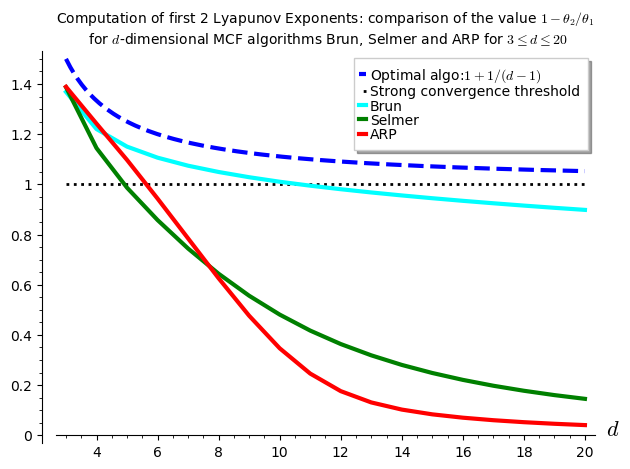
I have to say that I was disapointed by the results because the algorithm Arnoux-Rauzy-Poincaré (ARP) that Valérie and I introduced was not performing so well as its second Lyapunov exponent seems to become positive for dimension \(d\geq 6\). I had good expectations for ARP because it reaches the highest value for \(1-\theta_2/\theta_1\) in the computations performed in the Cheat Sheets, thus better than Brun, better than Selmer when \(d=3\).
The algorithm for the computation of the first two Lyapunov exponents was provided to me by Vincent Delecroix. It applies the algorithm \((v,w)\mapsto(M^{-1}v,M^T w)\) millions of times. The evolution of the size of the vector \(v\) gives the first Lyapunov exponent. The evolution of the size of the vector \(w\) gives the second Lyapunov exponent. Since the computation is performed on 64-bits double floating point number, their are numerical issues to deal with. This is why some Gramm Shimdts operation is performed on the vector \(w\) at each time the vectors are renormalized to keep the vector \(w\) orthogonal to \(v\). Otherwise, the numerical errors cumulate and the computed value for the \(\theta_2\) becomes the same as \(\theta_1\). You can look at the algorithm online starting at line 1723 of the file mult_cont_frac_pyx.pyx from my optional package.
I do not know from where Vincent took that algorithm. So, I do not know how exact it is and whether there exits any proof of lower bounds and upper bounds on the computations being performed. What I can say is that it is quite reliable in the sense that is returns the same values over and over again (by that I mean 3 common most significant digits) with any fixed inputs (number of iterations).
Below, I show the code illustrating how to reproduce the results.
The version 0.6 (November 2019) of my package slabbe includes the necessary code to deal with some \(d\)-dimensional Multidimensional Continued Fraction (MCF) algorithms. Its documentation is available online. It is a PIP package, so it can be installed like this:
sage -pip install slabbe
Recall that the dimension \(d\) below is the linear one and \(d-1\) is the dimension of the space for the corresponding projective algorithm.
Import the Brun, Selmer and Arnoux-Rauzy-Poincaré MCF algorithms from the optional package:
sage: from slabbe.mult_cont_frac import Brun, Selmer, ARP
The computation of the first two Lyapunov exponents performed on one single orbit:
sage: Brun(dim=3).lyapunov_exponents(n_iterations=10^7)
(0.30473782969922547, -0.11220958022368056, 1.3682167728713919)
The starting point is taken randomly, but the results of the form of a 3-tuple \((\theta_1,\theta_2,1-\theta_2/\theta_1)\) are about the same:
sage: Brun(dim=3).lyapunov_exponents(n_iterations=10^7)
(0.30345018206132324, -0.11171509867725296, 1.3681497170915415)
Increasing the dimension \(d\) yields:
sage: Brun(dim=4).lyapunov_exponents(n_iterations=10^7)
(0.32639514522732005, -0.07191456560115839, 1.2203297648654456)
sage: Brun(dim=5).lyapunov_exponents(n_iterations=10^7)
(0.30918877340506756, -0.0463930802132972, 1.1500477514185734)
It performs an orbit of length \(10^7\) in about .5 seconds, of length \(10^8\) in about 5 seconds and of length \(10^9\) in about 50 seconds:
sage: %time Brun(dim=3).lyapunov_exponents(n_iterations=10^7)
CPU times: user 540 ms, sys: 0 ns, total: 540 ms
Wall time: 539 ms
(0.30488799356325225, -0.11234354880132114, 1.3684748208296182)
sage: %time Brun(dim=3).lyapunov_exponents(n_iterations=10^8)
CPU times: user 5.09 s, sys: 0 ns, total: 5.09 s
Wall time: 5.08 s
(0.30455473631148755, -0.11217550411862384, 1.3683262505689446)
sage: %time Brun(dim=3).lyapunov_exponents(n_iterations=10^9)
CPU times: user 51.2 s, sys: 0 ns, total: 51.2 s
Wall time: 51.2 s
(0.30438755982577026, -0.11211562816821799, 1.368331834035505)
Here, in what follows, I must admit that I needed to do a small fix to my package, so the code below will not work in version 0.6 of my package, I will update my package in the next days in order that the computations below can be reproduced:
sage: from slabbe.lyapunov import lyapunov_comparison_table
For each \(3\leq d\leq 20\), I compute 30 orbits and I show the most significant digits and the standard deviation of the 30 values computed.
For Brun algorithm:
sage: algos = [Brun(d) for d in range(3,21)]
sage: %time lyapunov_comparison_table(algos, n_orbits=30, n_iterations=10^7, ncpus=8)
CPU times: user 190 ms, sys: 2.8 s, total: 2.99 s
Wall time: 6min 31s
  Algorithm     \#Orbits   $\theta_1$ (std)     $\theta_2$ (std)      $1-\theta_2/\theta_1$ (std)
+-------------+----------+--------------------+---------------------+-----------------------------+
  Brun (d=3)    30         0.3045 (0.00040)     -0.1122 (0.00017)     1.3683 (0.00022)
  Brun (d=4)    30         0.32632 (0.000055)   -0.07188 (0.000051)   1.2203 (0.00014)
  Brun (d=5)    30         0.30919 (0.000032)   -0.04647 (0.000041)   1.1503 (0.00013)
  Brun (d=6)    30         0.28626 (0.000027)   -0.03043 (0.000035)   1.1063 (0.00012)
  Brun (d=7)    30         0.26441 (0.000024)   -0.01966 (0.000027)   1.0743 (0.00010)
  Brun (d=8)    30         0.24504 (0.000027)   -0.01207 (0.000024)   1.04926 (0.000096)
  Brun (d=9)    30         0.22824 (0.000021)   -0.00649 (0.000026)   1.0284 (0.00012)
  Brun (d=10)   30         0.2138 (0.00098)     -0.0022 (0.00015)     1.0104 (0.00074)
  Brun (d=11)   30         0.20085 (0.000015)   0.00106 (0.000022)    0.9947 (0.00011)
  Brun (d=12)   30         0.18962 (0.000017)   0.00368 (0.000021)    0.9806 (0.00011)
  Brun (d=13)   30         0.17967 (0.000011)   0.00580 (0.000020)    0.9677 (0.00011)
  Brun (d=14)   30         0.17077 (0.000011)   0.00755 (0.000021)    0.9558 (0.00012)
  Brun (d=15)   30         0.16278 (0.000012)   0.00900 (0.000017)    0.9447 (0.00010)
  Brun (d=16)   30         0.15556 (0.000011)   0.01022 (0.000013)    0.93433 (0.000086)
  Brun (d=17)   30         0.149002 (9.5e-6)    0.01124 (0.000015)    0.9246 (0.00010)
  Brun (d=18)   30         0.14303 (0.000010)   0.01211 (0.000019)    0.9153 (0.00014)
  Brun (d=19)   30         0.13755 (0.000012)   0.01285 (0.000018)    0.9065 (0.00013)
  Brun (d=20)   30         0.13251 (0.000011)   0.01349 (0.000019)    0.8982 (0.00014)
For Selmer algorithm:
sage: algos = [Selmer(d) for d in range(3,21)]
sage: %time lyapunov_comparison_table(algos, n_orbits=30, n_iterations=10^7, ncpus=8)
CPU times: user 203 ms, sys: 2.78 s, total: 2.98 s
Wall time: 6min 27s
  Algorithm       \#Orbits   $\theta_1$ (std)     $\theta_2$ (std)      $1-\theta_2/\theta_1$ (std)
+---------------+----------+--------------------+---------------------+-----------------------------+
  Selmer (d=3)    30         0.1827 (0.00041)     -0.0707 (0.00017)     1.3871 (0.00029)
  Selmer (d=4)    30         0.15808 (0.000058)   -0.02282 (0.000036)   1.1444 (0.00023)
  Selmer (d=5)    30         0.13199 (0.000033)   0.00176 (0.000034)    0.9866 (0.00026)
  Selmer (d=6)    30         0.11205 (0.000017)   0.01595 (0.000036)    0.8577 (0.00031)
  Selmer (d=7)    30         0.09697 (0.000012)   0.02481 (0.000030)    0.7442 (0.00032)
  Selmer (d=8)    30         0.085340 (8.5e-6)    0.03041 (0.000032)    0.6437 (0.00036)
  Selmer (d=9)    30         0.076136 (5.9e-6)    0.03379 (0.000032)    0.5561 (0.00041)
  Selmer (d=10)   30         0.068690 (5.5e-6)    0.03565 (0.000023)    0.4810 (0.00032)
  Selmer (d=11)   30         0.062557 (4.4e-6)    0.03646 (0.000021)    0.4172 (0.00031)
  Selmer (d=12)   30         0.057417 (3.6e-6)    0.03654 (0.000017)    0.3636 (0.00028)
  Selmer (d=13)   30         0.05305 (0.000011)   0.03615 (0.000018)    0.3186 (0.00032)
  Selmer (d=14)   30         0.04928 (0.000060)   0.03546 (0.000051)    0.2804 (0.00040)
  Selmer (d=15)   30         0.046040 (2.0e-6)    0.03462 (0.000013)    0.2482 (0.00027)
  Selmer (d=16)   30         0.04318 (0.000011)   0.03365 (0.000014)    0.2208 (0.00028)
  Selmer (d=17)   30         0.040658 (3.3e-6)    0.03263 (0.000013)    0.1974 (0.00030)
  Selmer (d=18)   30         0.038411 (2.7e-6)    0.031596 (9.8e-6)     0.1774 (0.00022)
  Selmer (d=19)   30         0.036399 (2.2e-6)    0.030571 (8.0e-6)     0.1601 (0.00019)
  Selmer (d=20)   30         0.0346 (0.00011)     0.02955 (0.000093)    0.1452 (0.00019)
For Arnoux-Rauzy-Poincaré algorithm:
sage: algos = [ARP(d) for d in range(3,21)]
sage: %time lyapunov_comparison_table(algos, n_orbits=30, n_iterations=10^7, ncpus=8)
CPU times: user 226 ms, sys: 2.76 s, total: 2.99 s
Wall time: 13min 20s
  Algorithm                        \#Orbits   $\theta_1$ (std)     $\theta_2$ (std)      $1-\theta_2/\theta_1$ (std)
+--------------------------------+----------+--------------------+---------------------+-----------------------------+
  Arnoux-Rauzy-Poincar\'e (d=3)    30         0.4428 (0.00056)     -0.1722 (0.00025)     1.3888 (0.00016)
  Arnoux-Rauzy-Poincar\'e (d=4)    30         0.6811 (0.00020)     -0.16480 (0.000085)   1.24198 (0.000093)
  Arnoux-Rauzy-Poincar\'e (d=5)    30         0.7982 (0.00012)     -0.0776 (0.00010)     1.0972 (0.00013)
  Arnoux-Rauzy-Poincar\'e (d=6)    30         0.83563 (0.000091)   0.0475 (0.00010)      0.9432 (0.00012)
  Arnoux-Rauzy-Poincar\'e (d=7)    30         0.8363 (0.00011)     0.1802 (0.00016)      0.7845 (0.00020)
  Arnoux-Rauzy-Poincar\'e (d=8)    30         0.8213 (0.00013)     0.3074 (0.00023)      0.6257 (0.00028)
  Arnoux-Rauzy-Poincar\'e (d=9)    30         0.8030 (0.00012)     0.4205 (0.00017)      0.4763 (0.00022)
  Arnoux-Rauzy-Poincar\'e (d=10)   30         0.7899 (0.00011)     0.5160 (0.00016)      0.3467 (0.00020)
  Arnoux-Rauzy-Poincar\'e (d=11)   30         0.7856 (0.00014)     0.5924 (0.00020)      0.2459 (0.00022)
  Arnoux-Rauzy-Poincar\'e (d=12)   30         0.7883 (0.00010)     0.6497 (0.00012)      0.1759 (0.00014)
  Arnoux-Rauzy-Poincar\'e (d=13)   30         0.7930 (0.00010)     0.6892 (0.00014)      0.1309 (0.00014)
  Arnoux-Rauzy-Poincar\'e (d=14)   30         0.7962 (0.00012)     0.7147 (0.00015)      0.10239 (0.000077)
  Arnoux-Rauzy-Poincar\'e (d=15)   30         0.7974 (0.00012)     0.7309 (0.00014)      0.08340 (0.000074)
  Arnoux-Rauzy-Poincar\'e (d=16)   30         0.7969 (0.00015)     0.7411 (0.00014)      0.07010 (0.000048)
  Arnoux-Rauzy-Poincar\'e (d=17)   30         0.7960 (0.00014)     0.7482 (0.00014)      0.06005 (0.000050)
  Arnoux-Rauzy-Poincar\'e (d=18)   30         0.7952 (0.00013)     0.7537 (0.00014)      0.05218 (0.000046)
  Arnoux-Rauzy-Poincar\'e (d=19)   30         0.7949 (0.00012)     0.7584 (0.00013)      0.04582 (0.000035)
  Arnoux-Rauzy-Poincar\'e (d=20)   30         0.7948 (0.00014)     0.7626 (0.00013)      0.04058 (0.000025)
The computation of the figure shown above is done with the code below:
sage: brun_list = [1.3683, 1.2203, 1.1503, 1.1063, 1.0743, 1.04926, 1.0284, 1.0104, 0.9947, 0.9806, 0.9677, 0.9558, 0.9447, 0.93433, 0.9246, 0.9153, 0.9065, 0.8982]
sage: selmer_list = [ 1.3871, 1.1444, 0.9866, 0.8577, 0.7442, 0.6437, 0.5561, 0.4810, 0.4172, 0.3636, 0.3186, 0.2804, 0.2482, 0.2208, 0.1974, 0.1774, 0.1601, 0.1452]
sage: arp_list = [1.3888, 1.24198, 1.0972, 0.9432, 0.7845, 0.6257, 0.4763, 0.3467, 0.2459, 0.1759, 0.1309, 0.10239, 0.08340, 0.07010, 0.06005, 0.05218, 0.04582, 0.04058]
sage: brun_points = list(enumerate(brun_list, start=3))
sage: selmer_points = list(enumerate(selmer_list, start=3))
sage: arp_points = list(enumerate(arp_list, start=3))
sage: G = Graphics()
sage: G += plot(1+1/(x-1), x, 3, 20, legend_label='Optimal algo:$1+1/(d-1)$', linestyle='dashed', color='blue', thickness=3)
sage: G += line([(3,1), (20,1)], color='black', legend_label='Strong convergence threshold', linestyle='dotted', thickness=2)
sage: G += line(brun_points, legend_label='Brun', color='cyan', thickness=3)
sage: G += line(selmer_points, legend_label='Selmer', color='green', thickness=3)
sage: G += line(arp_points, legend_label='ARP', color='red', thickness=3)
sage: G.ymin(0)
sage: G.axes_labels(['$d$',''])
sage: G.show(title='Computation of first 2 Lyapunov Exponents: comparison of the value $1-\\theta_2/\\theta_1$\n for $d$-dimensional MCF algorithms Brun, Selmer and ARP for $3\\leq d\\leq 20$')
Propulsé par Blogofile
S'abonner au Flux RSS
et aux Commentaires.

This work by Sébastien Labbé is licensed under a Creative Commons Attribution-ShareAlike 4.0 International License.