Doron Zeilbeger made a talk last Friday at CRM in Montreal during Sage Days 38 about \(n^{n-2}\). At the end of the talk, he propoed a contest to code Joyal's Bijection which relates double rooted trees on \(n\) vertices and endofunctions on \(n\) elements. I wrote an implementation in Sage. My code is available here : joyal_bijection.sage. It will certainly not win for the most brief code, but it is object oriented, documented, reusable, testable and allows introspection.

sage: load joyal_bijection.sage

sage: L = [7, 0, 6, 1, 4, 7, 2, 1, 5]
sage: f = Endofunction(L)
sage: f
Endofunction:
[0..8] -> [7, 0, 6, 1, 4, 7, 2, 1, 5]

sage: L = [(0,6),(2,1),(3,1),(4,2),(5,7),(6,4),(7,0),(8,5)]
sage: D = DoubleRootedTree(L, 1, 7)
sage: D
Double rooted tree:
Edges: [(0, 6), (2, 1), (3, 1), (4, 2), (5, 7), (6, 4), (7, 0), (8, 5)]
RootA: 1
RootB: 7

sage: f.to_double_rooted_tree()
Double rooted tree:
Edges: [(0, 6), (2, 1), (3, 1), (4, 2), (5, 7), (6, 4), (7, 0), (8, 5)]
RootA: 1
RootB: 7

sage: D.to_endofunction()
Endofunction:
[0..8] -> [7, 0, 6, 1, 4, 7, 2, 1, 5]

sage: D == f.to_double_rooted_tree()
True
sage: f == D.to_endofunction()
True

sage: E = Endofunctions(10000)
sage: f = E.random_element()
sage: time f == f.to_double_rooted_tree().to_endofunction()
True
Time: CPU 2.23 s, Wall: 2.24 s

On December 21 2011, version 0.12 of IPython was released with its own notebook. The differences with the Sage Notebook are explained by Fernando Perez, leader of IPython project, in the blog post The IPython notebook: a historical retrospective he wrote last January. One of the differences is that the IPython Notebook run in its own directory whereas each cell of the Sage Notebook lives in its directory.

The latest version of IPython is 0.12.1 and was released in April 2012 and I was curious of testing it. I followed the installations informations. I got into trouble some times but finally managed to install it. Below is how I did to install IPython 0.12.1 on my OSX 10.5.8 using Python 2.6.7.

Installing dependencies:

sudo easy_install-2.6 tornado
sudo easy_install-2.6 nose
sudo easy_install-2.6 pyzmq

The following command was broken for a while:

sudo easy_install-2.6 pyzmq

ending with error TypeError: 'NoneType' object is not callable. I managed to make it work by redoing the above install commands in the correct above order:

sudo easy_install-2.6 tornado
sudo easy_install-2.6 nose
sudo easy_install-2.6 pyzmq

Installing ipython-0.12:

sudo easy_install-2.6 ipython

To make ipython known from the command line, I added the following line to the file ~/.bash_profile:

# ipython
export PATH=/opt/local/Library/Frameworks/Python.framework/Versions/2.6/bin:$PATH

I tested the ipython installation with the iptest command. It finishes with Status: OK

iptest

I open the ipython notebook and it worked:

ipython notebook
[NotebookApp] Using existing profile dir: u'/Users/slabbe/.ipython/profile_default'
[NotebookApp] The IPython Notebook is running at: http://127.0.0.1:8888
[NotebookApp] Use Control-C to stop this server and shut down all kernels.

In safari, I get the following problem:

Websocket connection to
ws://127.0.0.1:8888/kernels/86fef706-f386-4116-b3e4-d6d7776afb0d could not
be established.  You will NOT be able to run code.  Your browser may not be
compatible with the websocket version in the server, or if the url does not
look right, there could be an error in the server's configuration.

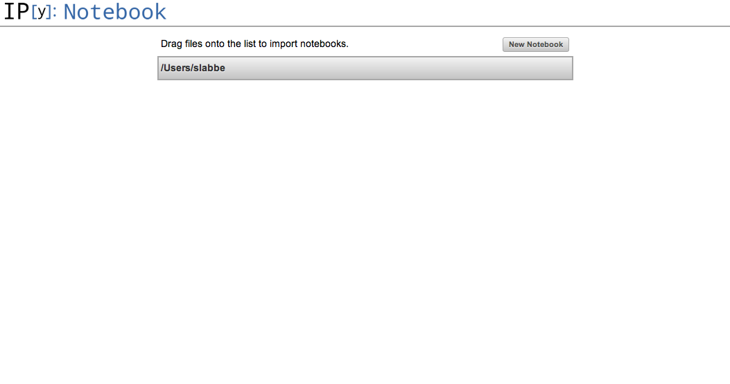
But, in firefox, it works when I open a page at the above adress http://127.0.0.1:8888. It gives me the following dashboard page.

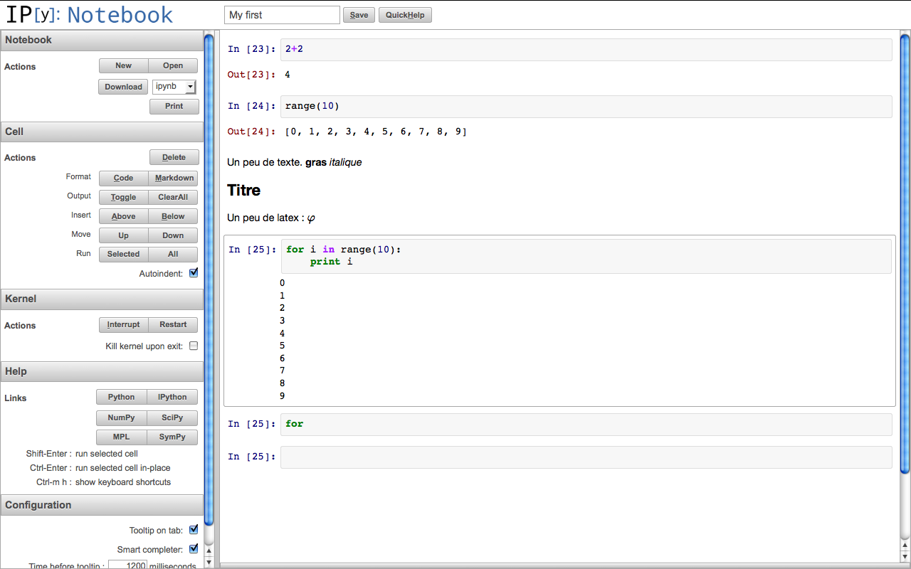
I created my first notebook and did some tests. I followed the documentation found here.

The next thing would be to try to use this with Sage. Some progress has been done and can be followed at ticket #12719.

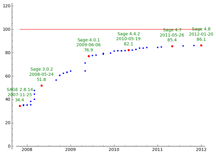
Recently, a discussion on sage-devel mentionned the graph I did last year for the evolution of the overall doctest coverage of Sage. The graph was out of date, so I updated it with the recent data:

Sage 4.7:   May 26, 2011        85.4%   ~  23769 / 27833
Sage 4.7.1: August 16, 2011     85.7%   ~  24129 / 28155
Sage 4.7.2: November 03, 2011   86.0%   ~  24477 / 28462
Sage 4.8:   January 20, 2012    86.1%   ~  24601 / 28573

We are far from the +4.7% a year I was expecting...

Doctest coverage of Sage

I think we should now stop looking at this percentage for the 100% coverage goal, because the coverage is mostly influenced by the hundreds of new doctested functions that are added to every new version of Sage.

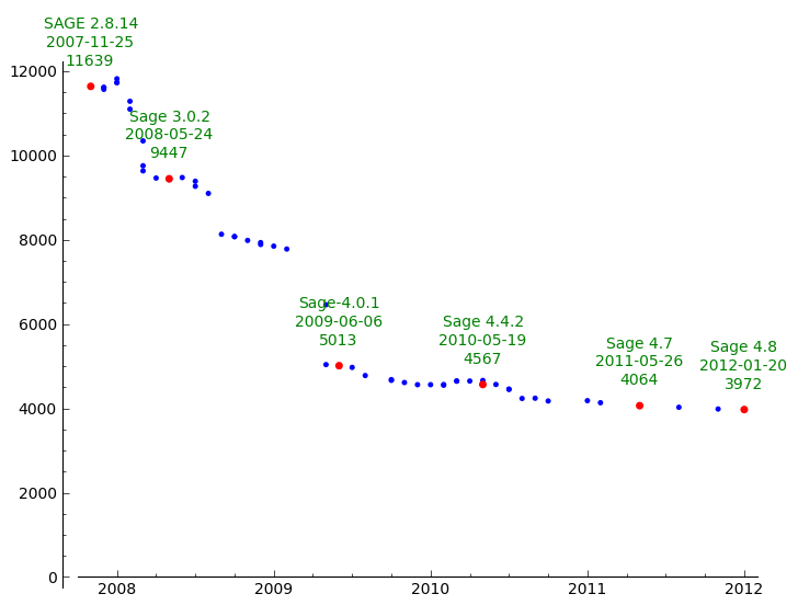
Instead we should consider the evolution of the number of undoctested functions (and maybe fix objectives about it):

Sage 4.7:   May 26, 2011        4064
Sage 4.7.1: August 16, 2011     4026  ->  38 old functions now 100% doctested
Sage 4.7.2: November 03, 2011   3985  ->  41 old functions now 100% doctested
Sage 4.8:   January 20, 2012    3972  ->  13 old functions now 100% doctested

Here is the graph of it:

Number of undoctested functions in Sage

Aujourd'hui, j'ai fait une présentation sur Sage au département de mathématiques du Cégep de Saint-Hyacinthe. Voici quelques liens.

La présentation (pdf) :

• sage-hyacinthe.pdf

Démo:

Les fichiers txt ci-bas peuvent être chargés à partir du bloc-note (Notebook) de Sage. Copier l'adresse et coller celle-ci dans la page Upload du bloc-note.

• cegep_st_hyacinthe_janvier_2012.txt
• tutoriel_sagenb_francais.txt
• tutoriel_python_francais.txt

Exercices :

1. Se créer un compte sur sagenb.org ou sur le serveur du LaCIM.
2. Faire un calcul de votre choix.
3. Trouver et tester un exemple de votre choix dans le tutoriel en français.
4. Trouver et tester un exemple de votre choix dans le wiki de Sage. Recherchez les liens Teaching with Sage, Interact ou Animation.
5. Importer (à partir de la page Upload) les feuilles de travail de démonstration ci-haut.
6. Consulter les feuilles de travail Sage publiées sur le serveur du LaCIM. Consulter celles indiquant MAT1112 - Chapitre 1 et MAT1112 - Chapitre 2. Je les ai créées à l'automne 2011 pour le cours de Calcul 1 que j'ai donné.

Livre :

• Le livre Calcul mathématique avec Sage. La nouvelle version, sortie en décembre 2011, comporte une centaine de pages de plus que la version précédente. C'est, sans contredit, la meilleure ressource sur Sage en français.

En Sage, il est relativement facile de créer des animations d'images en 2D. Pour cela, il suffit d'utiliser la commande animate qui s'occupera d'utiliser les commandes plus compliquées ffpmeg ou convert. Plusieurs exemples sont disponibles dans la documentation de Sage ou sur le wiki de Sage.

Par contre, il n'est pas encore possible de faire une animation d'objets graphiques 3D. Le logiciel Jmol, utilisé dans Sage pour faire de la visualisation 3D le permet, car les chimistes l'utilise pour faire des animations 3D de molécules complexes, mais cette fonctionalité n'a pas encore été exportée dans Sage. En juin dernier, j'en ai parlé à Jonathan Gutow, responsable des mises à jour de Jmol dans Sage, mais il doit d'abord régler d'autres problèmes plus importants.

En attendant, il est possible de s'en sortir en utilisant Tachyon plutôt que Jmol. Je rappelle que Tachyon est utilisé dans Sage pour créer des images png d'objets graphiques 3d. Ensuite, on peut immiter ce que la fonction animate fait pour créer une animation d'une scène 3d.

Pour illustrer la méthode par un exemple, faisons une animation de la technique des liens dansants de Knuth pour trouver les solutions du puzzle Quantumino.

Dans un répertoire, créer un fichier Sage video_quantumino.sage qui contiendra le code suivant:

from sage.games.quantumino import QuantuminoSolver
import itertools

def animate(block=4, stop=400, angle=pi/200.0, nb_pareil=5):
    r"""
    This functions creates plenty of png images in the images folder.

    INPUT:

    - ``block`` - integer between 0 and 16, the block to put aside

    - ``stop`` - integer, number of iterations

    - ``angle`` - number, rotation angle (radian) between each frame

    - ``nb_parei`` - integer, number of frame per iteration

    OUTPUT:

    Plenty of png images in the images folder.
    """
    q = QuantuminoSolver(block)
    it = q.solve(partial='incremental')
    i = 0
    for solution in itertools.islice(it, stop):
        G = solution.show3d()
        G += sphere((4,7,1),size=0.1,opacity=0) # hack to stabilize the frame
        G += sphere((0,7,0),size=0.1,opacity=0) # hack to stabilize the frame
        #G += sphere((2,4,1),size=10,opacity=0) # pas opaque pantoute

        for _ in range(nb_pareil):
            H = G.rotateZ(angle * i)

            filename = 'images/image%s.png' % i
            H.save(filename, frame=False, aspect_ratio=1)
            print "Création du fichier %s" % filename

            i += 1

animate(4, stop=20, angle=pi/200.0, nb_pareil=5)

Créer les images à l'aide de Sage >= 4.7.2

mkdir images
sage video_quantumino.sage

Aller dans le répertoire images et faites ensuite:

cd images
ffmpeg -y -f image2 -r 20 -i image%d.png video.mpg

Le résultat est ici (bloc numéro 4 mis de côté, 200 itérations, angle=\(\pi\)/200, 5 images par itérations, total de 1000 images):